> ## Documentation Index
> Fetch the complete documentation index at: https://docs.revilico.bio/llms.txt
> Use this file to discover all available pages before exploring further.
# RevPath
> Intrinsic reaction coordinate: follow a transition state downhill in both directions to see which minima it connects
## Why Use This Engine?
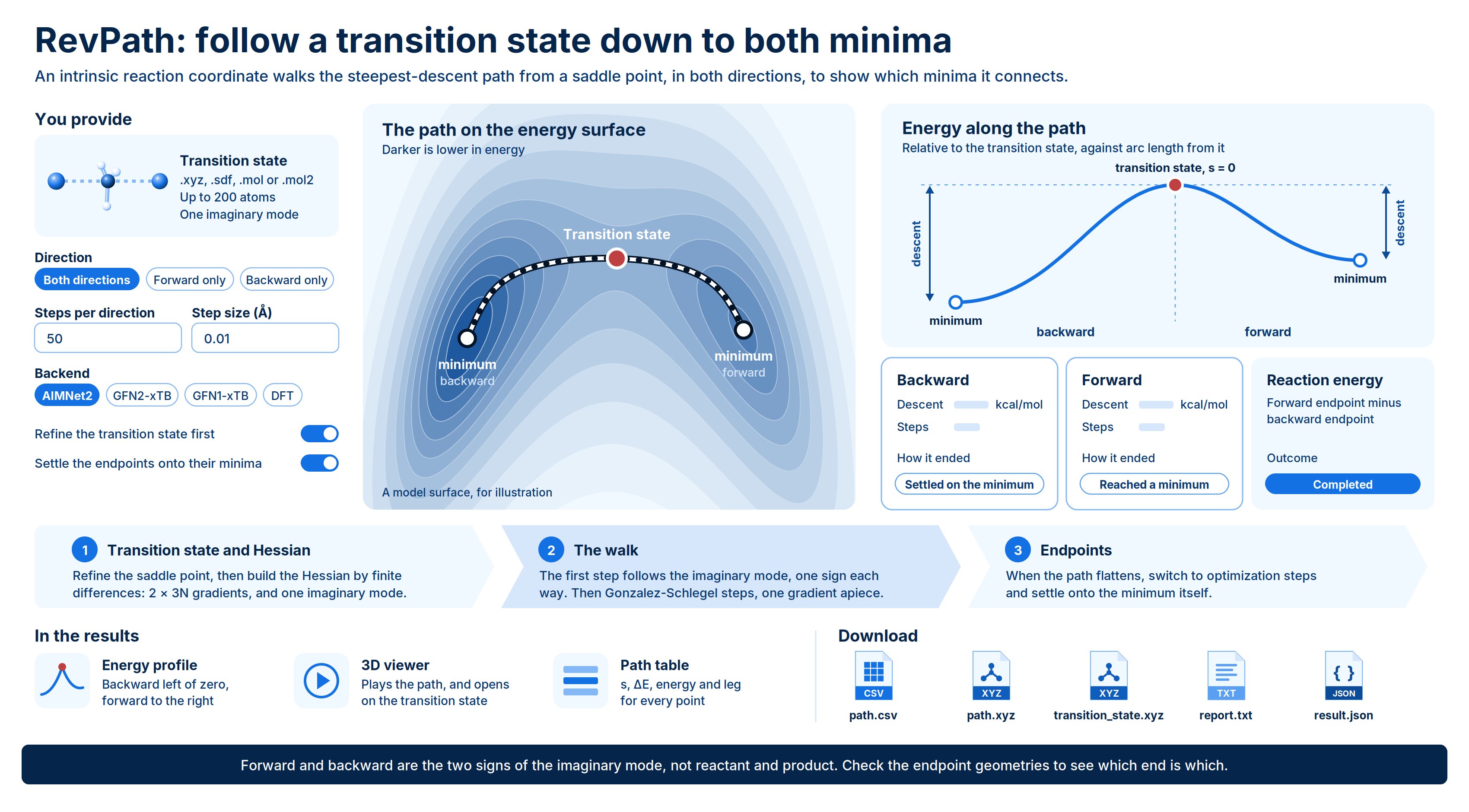
RevPath runs an intrinsic reaction coordinate (IRC) calculation. It starts from a transition state and walks the path of steepest descent in mass-weighted coordinates, in both directions, until each end reaches a minimum. The result is one continuous reaction path, running from one endpoint through the saddle point to the other, with an energy and a geometry at every point.
A converged transition state with one imaginary frequency tells you that a barrier exists. Only the path tells you whether it is the barrier between the two structures you think it is. Typical uses:
* **Confirm a transition state.** Check that a saddle point from [RevTS](/docs/revts) or another search connects the reactant and product you intended, and not some other pair of minima.
* **Read the barrier from both sides.** Each direction reports how far the energy falls from the transition state to its endpoint.
* **Get the reaction energy.** When both directions reach a minimum, RevPath reports the energy difference between the two endpoints.
* **Get a refined transition state.** With refinement on (the default), RevPath re-optimizes your saddle point at the chosen level of theory. You can download it on its own for follow-up calculations.
You submit one transition-state structure per run. You can choose a neural network potential, a semiempirical method or DFT to compute the energies.
 ## Background
An IRC is defined in mass-weighted Cartesian coordinates, $q_i = \sqrt{m_i}\, x_i$, where $m_i$ is the mass of the atom that coordinate belongs to. In these coordinates the reaction path is the curve of steepest descent from the saddle point:
$$
\frac{d\mathbf{q}}{ds} = -\frac{\mathbf{g}(\mathbf{q})}{\lVert \mathbf{g}(\mathbf{q}) \rVert}
$$
where $\mathbf{g}$ is the energy gradient with respect to the mass-weighted coordinates and $s$ is the arc length along the path, measured in Bohr·√amu. RevPath reports $s$ for every point, measured from the transition state.
A run has three stages:
1. **Transition state and Hessian.** The gradient is zero at a saddle point, so there is no downhill direction to follow yet. RevPath computes the Hessian (the matrix of second derivatives) by central finite differences, which costs $2 \times 3N$ gradient evaluations for $N$ atoms. The one negative eigenvalue of the Hessian gives the imaginary frequency and the reaction mode. A valid transition state has exactly one imaginary mode. The Hessian is computed once and reused by both directions.
2. **The walk.** The first step follows the imaginary-mode eigenvector, one sign for each direction. Every later step uses the Gonzalez-Schlegel method: move half a step along the gradient to a pivot point, then find the point on a sphere of half a step around the pivot where the gradient is parallel to the displacement. Each step costs one gradient evaluation.
3. **Endpoints.** When the path flattens out, each direction can switch to ordinary optimization steps so that it settles onto the minimum itself rather than stopping near it.
RevPath derives these quantities from the path:
* **Relative energy** of each point, relative to the transition state:
$$
\Delta E = \left( E - E_{\text{TS}} \right) \times 627.509 \ \text{kcal/mol per Hartree}
$$
It is negative everywhere along a well-behaved path, because the transition state is the maximum.
* **Descent** of each direction: $E_{\text{TS}} - E_{\text{endpoint}}$, in kcal/mol. This is the barrier seen from that endpoint. It is only a true barrier if that direction reached a minimum.
* **Reaction energy:** $E_{\text{forward endpoint}} - E_{\text{backward endpoint}}$, in kcal/mol. It is reported only when you run both directions and both reach a minimum.
**Forward** and **backward** are labels, not chemistry. They are the two signs of the imaginary-mode eigenvector, and which sign leads to your reactant is arbitrary. Do not assume that **forward** means products. For the same reason, the sign of the reaction energy follows the labels, not the direction of the reaction. Check the endpoint geometries to see which end is which.
## Validation
RevPath was benchmarked against a published third-party IRC calculation: the transition state for water adding to ethyl isocyanate (13 atoms, charge 0, singlet), at the reference's settings: GFN2-xTB, a 0.01 Å step and 50 steps in each direction. Transition-state refinement was off, because the reference geometry is already a converged saddle point and both calculations had to start from the same structure.
| Quantity | Reference | RevPath |
| - | - | - |
| Imaginary frequency | 1570.699i cm⁻¹ | 1570.714i cm⁻¹ |
| Larger descent | 19.6948 kcal/mol | 19.6961 kcal/mol |
| Smaller descent | 9.5748 kcal/mol | 9.5754 kcal/mol |
The descents agree to about 0.001 kcal/mol. They are compared as a pair, not by label, because the forward and backward labels are arbitrary (see the warning above).
The reference ran out of steps in both directions, so it does not test convergence to a minimum or endpoint optimization. Those are tested separately against an analytic model surface.
## Running the Engine
Open **Quantum Chemistry** > **RevQuant** > **RevPath**. The page has two tabs: **Reaction Path** to set up a run and **Analysis** to view results.
Enter a **Name** (optional, up to 200 characters). Runs without a name are named after their settings, for example `RevPath both, 50 steps at 0.01 Å`.
Drop a file on **Transition state**, or click to browse. You can also drag a file from the **Data Engineering** panel. Accepted formats are `.xyz`, `.sdf`, `.mol` and `.mol2`, up to 10 MB. The file must hold exactly one structure. See [Preparing the input file](#preparing-the-input-file).
Choose a **Direction**, the number of **Steps per direction** and the **Step size (Å)**. The defaults suit most transition states. See [Step size and step count](#step-size-and-step-count) if yours has a soft imaginary mode.
Select a **Backend**. For DFT, also choose a **Functional**; the form then shows an estimated runtime. Set the **Charge** and **Multiplicity** of the system.
Open **Advanced** to turn transition-state refinement or endpoint optimization on or off, choose an **Optimizer mode**, or choose a DFT **Basis set**.
Enter a **Runtime Limit (Credits)** to cap what the run can use. Leave it blank for no cap.
Click **Run reaction path**, then **Confirm**. A notification shows the estimated runtime, and the page switches to the **Analysis** tab with your run selected.
### Inputs
| Setting | Default | Options and notes |
| - | - | - |
| Name | Optional | Up to 200 characters |
| Transition state | Required | `.xyz`, `.sdf`, `.mol` or `.mol2`; one structure, up to 10 MB and 200 atoms |
| Direction | Both directions | Both directions, Forward only, Backward only |
| Steps per direction | 50 | 1 to 200. The limit applies to each direction separately, not to the total |
| Step size (Å) | 0.01 | 0.001 to 1 Å |
| Backend | AIMNet2 (ωB97M-D3) | AIMNet2 (ωB97M-D3), GFN2-xTB, GFN1-xTB, DFT (r²SCAN-D4 / ωB97M-D3BJ). See [Choosing a backend](#choosing-a-backend) |
| Functional | r²SCAN-D4 | DFT only. r²SCAN-D4 or ωB97M-D3BJ |
| Charge | 0 | -10 to 10 |
| Multiplicity | 1 | 1 to 11. Fixed at 1 for AIMNet2 |
| Refine the transition state first | On | A saddle-point search at the chosen backend before the walk |
| Settle the endpoints onto their minima | On | Switches to optimization steps once the path flattens |
| Optimizer mode | Standard | Draft (loosest, fastest), Standard, Fine, Ultrafine (slow), Exhaustive (very slow). Sets the convergence thresholds for the transition-state refinement and the endpoint optimization, not for the path steps |
| Basis set | def2-SVP | DFT only. def2-SVP, pcseg-1, def2-TZVP (about 5 times the wall-clock time of def2-SVP) |
| Runtime Limit (Credits) | No limit | Optional whole number. The run stops when it reaches the limit |
### Choosing a backend
| Backend | Type | Elements | Open shell | Notes |
| - | - | - | - | - |
| AIMNet2 (ωB97M-D3) | Neural network potential | H, B, C, N, O, F, Si, P, S, Cl, As, Se, Br, I | No | Recommended. Most accurate for organic molecules; an IRC runs in seconds |
| GFN2-xTB | Semiempirical | H to Rn, including transition metals | Yes | Use for elements AIMNet2 does not cover, or for open-shell systems |
| GFN1-xTB | Semiempirical | H to Rn | Yes | The older xTB parameterization. Prefer GFN2-xTB unless you are comparing against GFN1 results |
| DFT (r²SCAN-D4 / ωB97M-D3BJ) | Density functional theory | H to Rn, except the lanthanides Ce to Lu | Yes | Reference accuracy. Runs on a GPU and takes minutes to hours |
For DFT, **r²SCAN-D4** (a meta-GGA) is the routine choice. **ωB97M-D3BJ** (a hybrid) is the more accurate reference and costs more per gradient.
AIMNet2 has no spin channel, so it only runs closed-shell singlets and the **Multiplicity** field is locked to 1. Use an xTB or DFT backend for radicals and other open-shell systems.
A transition state belongs to the level of theory that produced it. A saddle point converged with one method is often not a saddle point at another; it can come back with several imaginary modes. Leave **Refine the transition state first** on unless the input was converged with the same backend and functional you are running. If the structure has more than one imaginary mode at the start of the walk, the run is refused.
### Preparing the input file
The file must contain one 3D structure: the transition state you want to walk from. A file with several structures, such as a multi-record SDF, is rejected, because it does not say which saddle point to use. Submit one run per transition state.
* **XYZ, SDF, MOL or MOL2.** The 3D coordinates are used as given, with hydrogens kept. A structure without 3D coordinates is rejected; a transition state is a specific geometry and cannot be generated from connectivity.
* **Charge and multiplicity** always come from the form, not from the file.
* **Elements** must be supported by the backend you choose (see [Choosing a backend](#choosing-a-backend)).
The structure should be an optimized transition state with one imaginary frequency. If it came from a cheaper method or a loose optimization, keep **Refine the transition state first** on.
### Step size and step count
The step size is a trust radius in Ångström. RevPath converts it to a mass-weighted step internally by scaling with the imaginary mode.
A transition state with a very soft imaginary mode, such as a hindered rotation, needs a **larger step, not more steps**. At the default 0.01 Å, a soft mode moves the geometry so little per step that the path can use its whole budget and go nowhere. On one 56i cm⁻¹ saddle point, seven steps in each direction moved the energy by less than 0.0001 kcal/mol. The optimizer also does not test for convergence until the path has covered roughly half an Ångström of mass-weighted displacement, so a path that barely moves cannot converge however many steps you allow.
If a direction runs out of steps while it is still clearly descending, increase **Steps per direction** instead.
### Run time and credits
The number of gradient evaluations in a run is fixed by the algorithm:
$$
\text{gradients} = 2 \times 3N + \text{path steps, all directions} + \text{number of directions}
$$
plus any transition-state refinement and endpoint optimization steps. The $2 \times 3N$ term is the Hessian, which is paid once whichever direction you choose. For a large molecule at DFT it is most of the job (61% of one 27-atom DFT run), so **Forward only** or **Backward only** roughly halves the path cost but not the total. Fewer steps cannot shrink the Hessian either.
As a guide:
| Backend | Typical run time |
| - | - |
| AIMNet2 | Seconds |
| GFN2-xTB, GFN1-xTB | Seconds to minutes |
| DFT | Minutes to hours |
For DFT on the GPU, r²SCAN-D4 takes about 5.8 seconds per gradient and ωB97M-D3BJ about 7.5 seconds, for a molecule with 279 basis functions at def2-SVP. Cost grows steeply with molecule size. DFT runs also go to a GPU queue that may take several minutes to start.
When you choose DFT, the form estimates the runtime from your structure, functional, direction and step count, and shows it before you submit. A DFT run has an 8-hour limit. If the estimate is over it, the form blocks the submission and suggests running one direction, using fewer steps, or choosing a faster backend. If the Hessian alone is over the limit, only a smaller molecule or a faster backend will help.
RevPath consumes 1 credit per minute of runtime while the calculation runs. You need enough credits to start a run. **Runtime Limit (Credits)** caps the total: if you set it, the run stops when it reaches that limit, with the status `terminated_budget_exceeded`. Leave it blank to run to completion without a cap. This credit limit is separate from the DFT time estimate described above.
## Viewing Results
Open the **Analysis** tab and click a run in the list. To pick a different run, click **Change Pipeline**. Results for runs that are still in progress refresh automatically every 10 seconds. While a run is working, the page notes that the transition state and its Hessian come first, then the walk.
### Run statuses
The status badge next to the run name is the status of the job:
| Status | Meaning |
| - | - |
| `not_started` | Submitted and waiting for compute |
| `started` | Running |
| `processed` | The job finished and wrote a reaction path. Check the outcome badge to see whether it reached its endpoints |
| `error` | The run produced no reaction path. The page shows the error message |
| `terminated_insufficient_credits` | Stopped because your credit balance ran out |
| `terminated_budget_exceeded` | Stopped because the run reached its **Runtime Limit (Credits)** |
A run fails with `error` if, for example, the input is not a first-order saddle point at the chosen backend, the file cannot be read, or the calculation crashes.
### Outcome
`processed` does not mean the IRC succeeded. A run whose directions ran out of steps still finishes as `processed`, because its path and files are real. Read the outcome badge in the results header to see what the run established.
| Outcome badge | Meaning |
| - | - |
| **Completed** | Every direction you ran reached an endpoint |
| **Incomplete** | At least one direction ran out of steps. The path is real as far as it goes, but it has not shown what the transition state connects to |
A run in which no direction produced a usable path finishes as `error` instead, with no results to show.
For an **Incomplete** run, a note above the results says which direction stalled and what to change. If the direction barely moved (less than 0.01 kcal/mol), increase the step size; the note also flags an imaginary mode below 200i cm⁻¹ as very soft. If the direction was still descending, increase the steps per direction.
### Results for a run
**Header.** The outcome badge, the number of path points, the imaginary frequency of the transition state (for example `saddle at 1570.7i cm⁻¹`), the total runtime, and **Download**.
**Direction and reaction energy cards.** One card per direction, showing its descent in kcal/mol, the number of steps and how it ended:
| Direction status | Meaning |
| - | - |
| Reached a minimum | Converged to a stationary point along the path |
| Settled on the minimum | The path flattened and endpoint optimization settled it onto the minimum |
| Ran out of steps | Used its whole step budget. The endpoint is wherever the walk stopped, not a minimum |
| Failed | The calculation gave up part-way along this direction |
The **Reaction energy** card shows the forward endpoint minus the backward endpoint in kcal/mol. It reads "not established" unless both directions reached a minimum.
**Energy profile.** Relative energy (kcal/mol) against the mass-weighted arc length from the transition state (Bohr·√amu). The backward direction is plotted to the left of zero and the forward direction to the right. The transition state is marked at zero, and each endpoint is labelled **minimum** or **ran out of steps**. Hover over a point to see its direction, step, relative energy, absolute energy and arc length. Click a point to show its geometry in the viewer.
The profile is plotted against arc length rather than step number because the step length adapts along the path, so equal step numbers are not equal distances.
**3D viewer.** Plays the path as a trajectory, from one endpoint through the transition state to the other. It opens on the transition state.
**Path table.** One row per point, in path order. Click a row to show that geometry in the viewer.
| Column | Values | Units |
| - | - | - |
| # | Position along the path | |
| s | Mass-weighted arc length from the transition state | Bohr·√amu |
| ΔE | Energy relative to the transition state | kcal/mol |
| Energy | Absolute energy | Hartree (Eh) |
| Leg | `backward` or `forward` and the step number, or **transition state** | |
### Downloads
Click **Download** in the results header. Each of these files opens in a new browser tab:
* **`path.csv`:** one row per path point, in path order. Columns: `index` (0-based position along the path), `direction` (`backward`, `forward` or `transition_state`), `step` (step number within its direction; 0 at the transition state), `arc_length_bohr_sqrt_amu`, `energy_hartree` and `relative_energy_kcal_per_mol`.
* **`path.xyz`:** the whole path as a multi-frame XYZ file, from one endpoint through the transition state to the other. Each frame's comment line gives its index, direction, step, arc length, energy (Eh) and relative energy (kcal/mol).
* **`transition_state.xyz`:** the transition-state geometry on its own, with its energy and imaginary frequency in the comment line. With refinement on, this is the refined saddle point, ready for follow-up calculations.
* **`report.txt`:** a plain-text summary: the settings and backend, the transition state (energy, imaginary frequency and number of imaginary modes, whether it was re-optimized, and the Hessian cost), each direction's steps, descent and status, the reaction energy if established, and a timing breakdown. It ends with a note if a direction ran out of steps.
* **`result.json`:** the full result document, including the request, every path point with its geometry, the transition state, each direction's result, the backend and model used, and timing.
## Limits
* One transition state per run, up to 200 atoms and 10 MB.
* Up to 200 steps per direction; step size from 0.001 to 1 Å.
* DFT runs are limited to 8 hours, and submissions estimated to exceed that are blocked.
* Gas phase only; solvation models are not available.
* AIMNet2 runs closed-shell singlets only.
* The input must be a first-order saddle point (exactly one imaginary mode) at the chosen backend, after refinement if refinement is on. RevPath does not search for transition states; use [RevTS](/docs/revts) or another method to find one first.
* A genuinely short reaction path, one that covers less than roughly half an Ångström of mass-weighted displacement, comes back **Incomplete** however many steps you allow.
* The forward and backward labels are arbitrary and do not identify reactants or products.
This documentation is built and hosted on [Mintlify](https://mintlify.com), a developer documentation platform.
## Background
An IRC is defined in mass-weighted Cartesian coordinates, $q_i = \sqrt{m_i}\, x_i$, where $m_i$ is the mass of the atom that coordinate belongs to. In these coordinates the reaction path is the curve of steepest descent from the saddle point:
$$
\frac{d\mathbf{q}}{ds} = -\frac{\mathbf{g}(\mathbf{q})}{\lVert \mathbf{g}(\mathbf{q}) \rVert}
$$
where $\mathbf{g}$ is the energy gradient with respect to the mass-weighted coordinates and $s$ is the arc length along the path, measured in Bohr·√amu. RevPath reports $s$ for every point, measured from the transition state.
A run has three stages:
1. **Transition state and Hessian.** The gradient is zero at a saddle point, so there is no downhill direction to follow yet. RevPath computes the Hessian (the matrix of second derivatives) by central finite differences, which costs $2 \times 3N$ gradient evaluations for $N$ atoms. The one negative eigenvalue of the Hessian gives the imaginary frequency and the reaction mode. A valid transition state has exactly one imaginary mode. The Hessian is computed once and reused by both directions.
2. **The walk.** The first step follows the imaginary-mode eigenvector, one sign for each direction. Every later step uses the Gonzalez-Schlegel method: move half a step along the gradient to a pivot point, then find the point on a sphere of half a step around the pivot where the gradient is parallel to the displacement. Each step costs one gradient evaluation.
3. **Endpoints.** When the path flattens out, each direction can switch to ordinary optimization steps so that it settles onto the minimum itself rather than stopping near it.
RevPath derives these quantities from the path:
* **Relative energy** of each point, relative to the transition state:
$$
\Delta E = \left( E - E_{\text{TS}} \right) \times 627.509 \ \text{kcal/mol per Hartree}
$$
It is negative everywhere along a well-behaved path, because the transition state is the maximum.
* **Descent** of each direction: $E_{\text{TS}} - E_{\text{endpoint}}$, in kcal/mol. This is the barrier seen from that endpoint. It is only a true barrier if that direction reached a minimum.
* **Reaction energy:** $E_{\text{forward endpoint}} - E_{\text{backward endpoint}}$, in kcal/mol. It is reported only when you run both directions and both reach a minimum.
**Forward** and **backward** are labels, not chemistry. They are the two signs of the imaginary-mode eigenvector, and which sign leads to your reactant is arbitrary. Do not assume that **forward** means products. For the same reason, the sign of the reaction energy follows the labels, not the direction of the reaction. Check the endpoint geometries to see which end is which.
## Validation
RevPath was benchmarked against a published third-party IRC calculation: the transition state for water adding to ethyl isocyanate (13 atoms, charge 0, singlet), at the reference's settings: GFN2-xTB, a 0.01 Å step and 50 steps in each direction. Transition-state refinement was off, because the reference geometry is already a converged saddle point and both calculations had to start from the same structure.
| Quantity | Reference | RevPath |
| - | - | - |
| Imaginary frequency | 1570.699i cm⁻¹ | 1570.714i cm⁻¹ |
| Larger descent | 19.6948 kcal/mol | 19.6961 kcal/mol |
| Smaller descent | 9.5748 kcal/mol | 9.5754 kcal/mol |
The descents agree to about 0.001 kcal/mol. They are compared as a pair, not by label, because the forward and backward labels are arbitrary (see the warning above).
The reference ran out of steps in both directions, so it does not test convergence to a minimum or endpoint optimization. Those are tested separately against an analytic model surface.
## Running the Engine
Open **Quantum Chemistry** > **RevQuant** > **RevPath**. The page has two tabs: **Reaction Path** to set up a run and **Analysis** to view results.
Enter a **Name** (optional, up to 200 characters). Runs without a name are named after their settings, for example `RevPath both, 50 steps at 0.01 Å`.
Drop a file on **Transition state**, or click to browse. You can also drag a file from the **Data Engineering** panel. Accepted formats are `.xyz`, `.sdf`, `.mol` and `.mol2`, up to 10 MB. The file must hold exactly one structure. See [Preparing the input file](#preparing-the-input-file).
Choose a **Direction**, the number of **Steps per direction** and the **Step size (Å)**. The defaults suit most transition states. See [Step size and step count](#step-size-and-step-count) if yours has a soft imaginary mode.
Select a **Backend**. For DFT, also choose a **Functional**; the form then shows an estimated runtime. Set the **Charge** and **Multiplicity** of the system.
Open **Advanced** to turn transition-state refinement or endpoint optimization on or off, choose an **Optimizer mode**, or choose a DFT **Basis set**.
Enter a **Runtime Limit (Credits)** to cap what the run can use. Leave it blank for no cap.
Click **Run reaction path**, then **Confirm**. A notification shows the estimated runtime, and the page switches to the **Analysis** tab with your run selected.
### Inputs
| Setting | Default | Options and notes |
| - | - | - |
| Name | Optional | Up to 200 characters |
| Transition state | Required | `.xyz`, `.sdf`, `.mol` or `.mol2`; one structure, up to 10 MB and 200 atoms |
| Direction | Both directions | Both directions, Forward only, Backward only |
| Steps per direction | 50 | 1 to 200. The limit applies to each direction separately, not to the total |
| Step size (Å) | 0.01 | 0.001 to 1 Å |
| Backend | AIMNet2 (ωB97M-D3) | AIMNet2 (ωB97M-D3), GFN2-xTB, GFN1-xTB, DFT (r²SCAN-D4 / ωB97M-D3BJ). See [Choosing a backend](#choosing-a-backend) |
| Functional | r²SCAN-D4 | DFT only. r²SCAN-D4 or ωB97M-D3BJ |
| Charge | 0 | -10 to 10 |
| Multiplicity | 1 | 1 to 11. Fixed at 1 for AIMNet2 |
| Refine the transition state first | On | A saddle-point search at the chosen backend before the walk |
| Settle the endpoints onto their minima | On | Switches to optimization steps once the path flattens |
| Optimizer mode | Standard | Draft (loosest, fastest), Standard, Fine, Ultrafine (slow), Exhaustive (very slow). Sets the convergence thresholds for the transition-state refinement and the endpoint optimization, not for the path steps |
| Basis set | def2-SVP | DFT only. def2-SVP, pcseg-1, def2-TZVP (about 5 times the wall-clock time of def2-SVP) |
| Runtime Limit (Credits) | No limit | Optional whole number. The run stops when it reaches the limit |
### Choosing a backend
| Backend | Type | Elements | Open shell | Notes |
| - | - | - | - | - |
| AIMNet2 (ωB97M-D3) | Neural network potential | H, B, C, N, O, F, Si, P, S, Cl, As, Se, Br, I | No | Recommended. Most accurate for organic molecules; an IRC runs in seconds |
| GFN2-xTB | Semiempirical | H to Rn, including transition metals | Yes | Use for elements AIMNet2 does not cover, or for open-shell systems |
| GFN1-xTB | Semiempirical | H to Rn | Yes | The older xTB parameterization. Prefer GFN2-xTB unless you are comparing against GFN1 results |
| DFT (r²SCAN-D4 / ωB97M-D3BJ) | Density functional theory | H to Rn, except the lanthanides Ce to Lu | Yes | Reference accuracy. Runs on a GPU and takes minutes to hours |
For DFT, **r²SCAN-D4** (a meta-GGA) is the routine choice. **ωB97M-D3BJ** (a hybrid) is the more accurate reference and costs more per gradient.
AIMNet2 has no spin channel, so it only runs closed-shell singlets and the **Multiplicity** field is locked to 1. Use an xTB or DFT backend for radicals and other open-shell systems.
A transition state belongs to the level of theory that produced it. A saddle point converged with one method is often not a saddle point at another; it can come back with several imaginary modes. Leave **Refine the transition state first** on unless the input was converged with the same backend and functional you are running. If the structure has more than one imaginary mode at the start of the walk, the run is refused.
### Preparing the input file
The file must contain one 3D structure: the transition state you want to walk from. A file with several structures, such as a multi-record SDF, is rejected, because it does not say which saddle point to use. Submit one run per transition state.
* **XYZ, SDF, MOL or MOL2.** The 3D coordinates are used as given, with hydrogens kept. A structure without 3D coordinates is rejected; a transition state is a specific geometry and cannot be generated from connectivity.
* **Charge and multiplicity** always come from the form, not from the file.
* **Elements** must be supported by the backend you choose (see [Choosing a backend](#choosing-a-backend)).
The structure should be an optimized transition state with one imaginary frequency. If it came from a cheaper method or a loose optimization, keep **Refine the transition state first** on.
### Step size and step count
The step size is a trust radius in Ångström. RevPath converts it to a mass-weighted step internally by scaling with the imaginary mode.
A transition state with a very soft imaginary mode, such as a hindered rotation, needs a **larger step, not more steps**. At the default 0.01 Å, a soft mode moves the geometry so little per step that the path can use its whole budget and go nowhere. On one 56i cm⁻¹ saddle point, seven steps in each direction moved the energy by less than 0.0001 kcal/mol. The optimizer also does not test for convergence until the path has covered roughly half an Ångström of mass-weighted displacement, so a path that barely moves cannot converge however many steps you allow.
If a direction runs out of steps while it is still clearly descending, increase **Steps per direction** instead.
### Run time and credits
The number of gradient evaluations in a run is fixed by the algorithm:
$$
\text{gradients} = 2 \times 3N + \text{path steps, all directions} + \text{number of directions}
$$
plus any transition-state refinement and endpoint optimization steps. The $2 \times 3N$ term is the Hessian, which is paid once whichever direction you choose. For a large molecule at DFT it is most of the job (61% of one 27-atom DFT run), so **Forward only** or **Backward only** roughly halves the path cost but not the total. Fewer steps cannot shrink the Hessian either.
As a guide:
| Backend | Typical run time |
| - | - |
| AIMNet2 | Seconds |
| GFN2-xTB, GFN1-xTB | Seconds to minutes |
| DFT | Minutes to hours |
For DFT on the GPU, r²SCAN-D4 takes about 5.8 seconds per gradient and ωB97M-D3BJ about 7.5 seconds, for a molecule with 279 basis functions at def2-SVP. Cost grows steeply with molecule size. DFT runs also go to a GPU queue that may take several minutes to start.
When you choose DFT, the form estimates the runtime from your structure, functional, direction and step count, and shows it before you submit. A DFT run has an 8-hour limit. If the estimate is over it, the form blocks the submission and suggests running one direction, using fewer steps, or choosing a faster backend. If the Hessian alone is over the limit, only a smaller molecule or a faster backend will help.
RevPath consumes 1 credit per minute of runtime while the calculation runs. You need enough credits to start a run. **Runtime Limit (Credits)** caps the total: if you set it, the run stops when it reaches that limit, with the status `terminated_budget_exceeded`. Leave it blank to run to completion without a cap. This credit limit is separate from the DFT time estimate described above.
## Viewing Results
Open the **Analysis** tab and click a run in the list. To pick a different run, click **Change Pipeline**. Results for runs that are still in progress refresh automatically every 10 seconds. While a run is working, the page notes that the transition state and its Hessian come first, then the walk.
### Run statuses
The status badge next to the run name is the status of the job:
| Status | Meaning |
| - | - |
| `not_started` | Submitted and waiting for compute |
| `started` | Running |
| `processed` | The job finished and wrote a reaction path. Check the outcome badge to see whether it reached its endpoints |
| `error` | The run produced no reaction path. The page shows the error message |
| `terminated_insufficient_credits` | Stopped because your credit balance ran out |
| `terminated_budget_exceeded` | Stopped because the run reached its **Runtime Limit (Credits)** |
A run fails with `error` if, for example, the input is not a first-order saddle point at the chosen backend, the file cannot be read, or the calculation crashes.
### Outcome
`processed` does not mean the IRC succeeded. A run whose directions ran out of steps still finishes as `processed`, because its path and files are real. Read the outcome badge in the results header to see what the run established.
| Outcome badge | Meaning |
| - | - |
| **Completed** | Every direction you ran reached an endpoint |
| **Incomplete** | At least one direction ran out of steps. The path is real as far as it goes, but it has not shown what the transition state connects to |
A run in which no direction produced a usable path finishes as `error` instead, with no results to show.
For an **Incomplete** run, a note above the results says which direction stalled and what to change. If the direction barely moved (less than 0.01 kcal/mol), increase the step size; the note also flags an imaginary mode below 200i cm⁻¹ as very soft. If the direction was still descending, increase the steps per direction.
### Results for a run
**Header.** The outcome badge, the number of path points, the imaginary frequency of the transition state (for example `saddle at 1570.7i cm⁻¹`), the total runtime, and **Download**.
**Direction and reaction energy cards.** One card per direction, showing its descent in kcal/mol, the number of steps and how it ended:
| Direction status | Meaning |
| - | - |
| Reached a minimum | Converged to a stationary point along the path |
| Settled on the minimum | The path flattened and endpoint optimization settled it onto the minimum |
| Ran out of steps | Used its whole step budget. The endpoint is wherever the walk stopped, not a minimum |
| Failed | The calculation gave up part-way along this direction |
The **Reaction energy** card shows the forward endpoint minus the backward endpoint in kcal/mol. It reads "not established" unless both directions reached a minimum.
**Energy profile.** Relative energy (kcal/mol) against the mass-weighted arc length from the transition state (Bohr·√amu). The backward direction is plotted to the left of zero and the forward direction to the right. The transition state is marked at zero, and each endpoint is labelled **minimum** or **ran out of steps**. Hover over a point to see its direction, step, relative energy, absolute energy and arc length. Click a point to show its geometry in the viewer.
The profile is plotted against arc length rather than step number because the step length adapts along the path, so equal step numbers are not equal distances.
**3D viewer.** Plays the path as a trajectory, from one endpoint through the transition state to the other. It opens on the transition state.
**Path table.** One row per point, in path order. Click a row to show that geometry in the viewer.
| Column | Values | Units |
| - | - | - |
| # | Position along the path | |
| s | Mass-weighted arc length from the transition state | Bohr·√amu |
| ΔE | Energy relative to the transition state | kcal/mol |
| Energy | Absolute energy | Hartree (Eh) |
| Leg | `backward` or `forward` and the step number, or **transition state** | |
### Downloads
Click **Download** in the results header. Each of these files opens in a new browser tab:
* **`path.csv`:** one row per path point, in path order. Columns: `index` (0-based position along the path), `direction` (`backward`, `forward` or `transition_state`), `step` (step number within its direction; 0 at the transition state), `arc_length_bohr_sqrt_amu`, `energy_hartree` and `relative_energy_kcal_per_mol`.
* **`path.xyz`:** the whole path as a multi-frame XYZ file, from one endpoint through the transition state to the other. Each frame's comment line gives its index, direction, step, arc length, energy (Eh) and relative energy (kcal/mol).
* **`transition_state.xyz`:** the transition-state geometry on its own, with its energy and imaginary frequency in the comment line. With refinement on, this is the refined saddle point, ready for follow-up calculations.
* **`report.txt`:** a plain-text summary: the settings and backend, the transition state (energy, imaginary frequency and number of imaginary modes, whether it was re-optimized, and the Hessian cost), each direction's steps, descent and status, the reaction energy if established, and a timing breakdown. It ends with a note if a direction ran out of steps.
* **`result.json`:** the full result document, including the request, every path point with its geometry, the transition state, each direction's result, the backend and model used, and timing.
## Limits
* One transition state per run, up to 200 atoms and 10 MB.
* Up to 200 steps per direction; step size from 0.001 to 1 Å.
* DFT runs are limited to 8 hours, and submissions estimated to exceed that are blocked.
* Gas phase only; solvation models are not available.
* AIMNet2 runs closed-shell singlets only.
* The input must be a first-order saddle point (exactly one imaginary mode) at the chosen backend, after refinement if refinement is on. RevPath does not search for transition states; use [RevTS](/docs/revts) or another method to find one first.
* A genuinely short reaction path, one that covers less than roughly half an Ångström of mass-weighted displacement, comes back **Incomplete** however many steps you allow.
* The forward and backward labels are arbitrary and do not identify reactants or products.
This documentation is built and hosted on [Mintlify](https://mintlify.com), a developer documentation platform.