RevSingleCell

Documentation Index

Fetch the complete documentation index at: https://docs.revilico.bio/llms.txt

Use this file to discover all available pages before exploring further.

​

Why Use This Engine?

In the documentation below, we will use Revilico’s Single Cell RNA sequencing analysis engine to explore and interpret a disease state from a transcriptomic perspective and evaluate whether a particular gene can serve as a potential therapeutic target.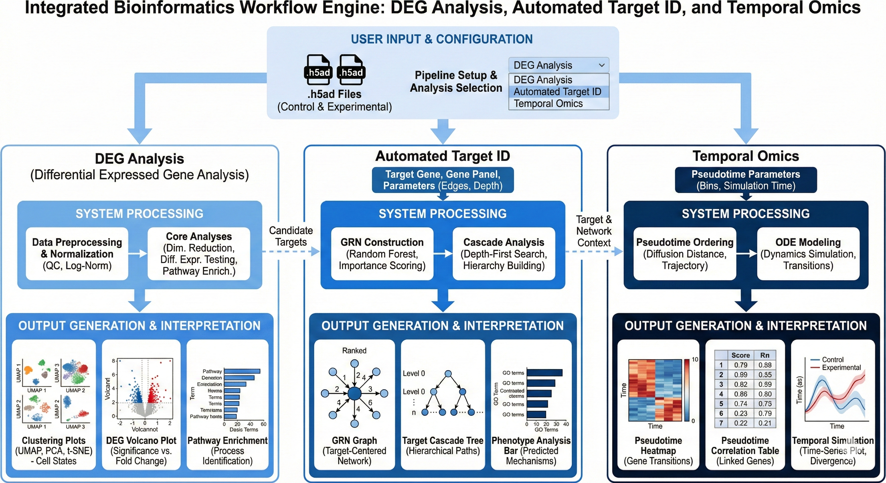

​

Background

Transcriptomics is the study of an organism’s RNA molecules at a specific time in order to derive insights such as gene expression and gene regulation in many different scenarios ranging from cellular function to comprehension of a disease state. One type of transcriptomic technology in particular is Single Cell RNA sequencing, which is a powerful technique where gene expression of several transcripts can be measured in each individual cell across thousands of cells, allowing users to screen cells of different conditions at a high throughput level. Revilico’s scRNA-seq Analysis Engine integrates 3 different workflows where the user can do the following: (1) perform genome-wide differential expression screening (DEG Analysis), (2) evaluate therapeutic target candidates through gene regulatory network analysis, regulatory correlation mapping, and downstream cascade prediction (Automated Target ID), and (3) model dynamic gene expression transitions using pseudotime trajectory inference coupled with RNA velocity-based temporal modeling (Temporal Omics Analysis). We will explain these in greater detail below. This engine supports hypothesis generation, target validation, and mechanistic understanding of perturbation responses in biological systems. Before diving into each workflow, we will first describe the core preprocessing pipeline that runs at the beginning of every analysis, as these steps are foundational to all three workflows described above.

​

Core Preprocessing Pipeline

​

1. Data Loading and Format Support

The engine accepts several common single-cell data formats: .h5ad (native AnnData), .h5 (10x Genomics HDF5 or generic HDF5), and count matrix files (.csv, .tsv, .txt). When performing differential expression between conditions, the user supplies both a control dataset and an experimental dataset. The engine concatenates these into a single AnnData object and assigns a condition label (control or experimental) to each cell in the observation metadata. This label is then used downstream during DEG analysis to group cells by biological condition rather than by cluster alone.

​

2. Quality Control

Once data is loaded, quality control filtering is applied to remove low-quality cells and uninformative genes. The engine computes the following per-cell metrics: number of detected genes, total UMI count, and the fraction of reads mapping to mitochondrial genes (genes whose names begin with “MT-”). Cells with fewer than min_genes or more than max_genes detected genes are removed, cells exceeding max_pct_mt percent mitochondrial content are removed, and genes detected in fewer than 3 cells are removed. The default thresholds are min_genes = 200, max_genes = 6000, and max_pct_mt = 20%. After filtering, QC summary metrics are reported including cells before and after filtering, median genes per cell, median UMI per cell, and median mitochondrial percentage. Optionally, doublet detection can be enabled via Scrublet, which flags likely multiplets before downstream analysis.

​

3. Normalization and Highly Variable Gene Selection

After QC, the raw count matrix is normalized so that each cell sums to 10,000 counts (counts per million scaling), then log-transformed: $$\tilde{x}_{ij} = \log\left(\frac{x_{ij}}{\sum_{j} x_{ij}} \cdot 10000 + 1\right)$$ Where $x_{ij}$ is the raw count for gene $j$ in cell $i$ and $\tilde{x}_{ij}$ is the normalized log expression. The raw counts are preserved in adata.raw before any gene selection or scaling occurs. Highly variable genes (HVGs) are then selected using a mean-dispersion approach adapted from Seurat, retaining the top 2,000 genes with the highest normalized dispersion relative to their mean expression. Gene expression is then scaled to zero mean with a maximum value cap of 10 to prevent outlier genes from dominating variance decomposition. Optionally, the engine can regress out technical covariates (total UMI count and mitochondrial percentage) before scaling, which is useful when these variables are expected to confound the biological signal of interest.

​

4. Dimensionality Reduction

Principal Component Analysis (PCA) is applied to the scaled HVG matrix using an ARPACK sparse solver, extracting up to 50 principal components. The number of components is automatically capped at min(n_cells - 1, n_genes). A k-nearest neighbor graph is then constructed in PCA space using 15 neighbors and 40 PCs, followed by UMAP embedding for 2D visualization. If the user provides a batch key column in the cell metadata, Harmony batch correction is applied to the PCA embedding before neighbor graph construction. Harmony iteratively adjusts the PCA coordinates so that cells from different batches intermix based on biological identity rather than technical origin. The UMAP is recomputed on the Harmony-corrected representation, and both the original and corrected UMAPs are retained for comparison.

​

5. Clustering and Cell Type Annotation

The engine runs both Leiden and Louvain graph-based clustering algorithms on the neighbor graph. The resolution parameter (default 0.5) controls cluster granularity; higher values produce more fine-grained clusters. Leiden clustering is used as the primary cluster label throughout downstream analyses. For each cluster, the top 50 marker genes are identified using a Wilcoxon rank-sum test against all remaining cells, ranked by test statistic. Cell type annotation is then performed by scoring the overlap between each cluster’s marker genes and a curated database of canonical marker genes spanning immune cell types, stromal cells, epithelial cells, and neurons. The engine also handles gene identifiers in Ensembl format (ENSG, ENSMUSG) by converting them to gene symbols via the MyGeneInfo API or the Ensembl REST API before annotation. The cell type with the highest enrichment score against the marker database is assigned to each cluster.

​

DEG Analysis

​

Overview

The DEG Analysis workflow performs genome-wide differential expression testing between two biological conditions (e.g. treated vs. untreated, disease vs. healthy). The user uploads a control dataset and an experimental dataset, and the engine identifies which genes are significantly upregulated or downregulated in the experimental condition. The results include a ranked list of DEGs per group, a volcano plot, and a heatmap of the top differentially expressed genes.

​

Wilcoxon Rank-Sum Test

By default, the engine uses the Wilcoxon rank-sum test (also called the Mann-Whitney U test) for differential expression. This is a non-parametric test that is well suited to the count-based, overdispersed distributions of scRNA-seq data. For each gene, cells in each group are ranked by expression, and the test statistic $U$ is computed as: $$U = R_1 - \frac{n_1(n_1 + 1)}{2}$$ Where $R_1$ is the sum of ranks for cells in group 1 and $n_1$ is the number of cells in group 1. The normalized test statistic is then converted to a p-value. All p-values are corrected for multiple testing using the Benjamini-Hochberg false discovery rate procedure. As an alternative to the Wilcoxon test, the user can select a t-test for cases where parametric assumptions are acceptable. Log fold-change between groups is computed on the log-normalized expression values: $$\text{logFC} = \overline{\log(x_{\text{exp}} + 1)} - \overline{\log(x_{\text{ctrl}} + 1)}$$ Where $\overline{\log(x_{\text{exp}} + 1)}$ and $\overline{\log(x_{\text{ctrl}} + 1)}$ are the mean log-normalized expression values in the experimental and control groups, respectively. Genes with adjusted p-value below 0.05 are considered statistically significant. The engine reports separately the number of significantly upregulated genes (logFC > 0) and significantly downregulated genes (logFC < 0).

​

Grouping Strategy

When the user provides both a control and experimental dataset, DEG analysis is grouped by condition (control vs. experimental). If only a single dataset is provided, DEG analysis is performed per Leiden cluster against all other cells, which is equivalent to marker gene detection at the condition level.

​

Outputs

• Volcano plot: Each gene is plotted with logFC on the x-axis and -log10(adjusted p-value) on the y-axis, colored by significance status
• DEG heatmap: Mean expression of the top differentially expressed genes per group, visualized as a clustered heatmap
• DEG table: Per-group ranked list of genes with score, adjusted p-value, and logFC

​

Automated Target ID

​

Overview

Automated Target ID builds on the DEG results to evaluate which differentially expressed genes are viable therapeutic targets. This workflow combines gene regulatory network analysis, regulatory correlation mapping, and downstream cascade prediction using transcription factor activity inference, pathway activity inference, and druggability annotation. The goal is to move from a ranked list of DEGs to a prioritized set of target candidates with mechanistic context.

​

Transcription Factor Activity Inference (Regulatory Network Analysis)

Rather than relying on raw gene expression alone, the engine estimates transcription factor (TF) activity at the single-cell level using the Univariate Linear Model (ULM) method from the decoupler library. TF activity scores reflect how strongly a TF’s known regulon is coordinately expressed in each cell, providing a more robust regulatory signal than the expression of the TF gene itself. The TF-target interaction network is sourced from Dorothea, a curated database of human TF-target interactions at confidence levels A through C. For each TF $t$ and cell $c$, ULM fits the following linear model: $$y_c = a_t \cdot x_{t,c} + \varepsilon_c$$ Where $y_c$ is the per-cell expression of all target genes in the regulon, $x_{t,c}$ is the prior weight (regulatory sign and confidence) of each target gene under TF $t$, $a_t$ is the estimated activity coefficient, and $\varepsilon_c$ is the residual. The activity score reported for each TF is the t-statistic of the coefficient $a_t$, which captures both the magnitude and consistency of regulon induction. Positive scores indicate that the TF’s activating targets are coordinately upregulated; negative scores indicate that the TF’s repressive program is engaged. Raw counts are used when available (from adata.raw) for this calculation to preserve the original signal.

​

Pathway Activity Inference (Regulatory Correlation Mapping)

Pathway activity is estimated using the Multivariate Linear Model (MLM) from decoupler, applied to the PROGENy signaling pathway network. PROGENy is derived from a large compendium of perturbation experiments and provides a set of gene-level footprint weights for 14 core signaling pathways including EGFR, MAPK, PI3K, TGFb, TNF, WNT, and others. For each pathway $p$ and cell $c$: $$\mathbf{y}_c = \mathbf{X} \cdot \boldsymbol{\beta}_p + \boldsymbol{\varepsilon}_c$$ Where $\mathbf{y}_c$ is the vector of expression values for pathway footprint genes in cell $c$, $\mathbf{X}$ contains the PROGENy weights for pathway $p$ (top 500 response genes), and $\boldsymbol{\beta}_p$ is estimated by ordinary least squares. The estimated coefficient $\beta_p$ serves as the per-cell pathway activity score. This approach links the observed transcriptional state of each cell to the activity of specific upstream signaling cascades, allowing the user to identify which pathways are most perturbed in the experimental condition and whether a target gene sits at the nexus of active regulatory networks.

​

Downstream Cascade Prediction and Target Annotation

The top DEGs ranked by absolute logFC are queried against the MyGeneInfo API to retrieve structured biological annotations for each candidate target. For each gene, the engine retrieves the gene name and functional summary, associated KEGG pathways (top 3), Gene Ontology Biological Process terms, and the Pharos druggability tier (TDL). Pharos classifies targets into four tiers: Tclin (approved drug target), Tchem (has known small molecule ligands), Tbio (biologically characterized but not yet drugged), and Tdark (little known biology). This classification directly informs target tractability. The combination of TF activity scores, pathway activity scores, and druggability annotation constitutes the regulatory context layer for each DEG. A gene that is differentially expressed, sits downstream of an active TF regulon, is linked to a perturbed signaling pathway, and has a favorable Pharos tier represents a well-supported therapeutic candidate.

​

Outputs

• TF activity heatmap: Per-cell TF activity scores across inferred TFs, shown as a heatmap
• TF activity UMAP: UMAP embeddings colored by individual TF activity scores
• Pathway activity heatmap: Per-cell pathway activity scores across the 14 PROGENy pathways
• Pathway activity UMAP: UMAP colored by individual pathway activity
• Target table: Annotated list of top candidate targets with KEGG pathways, GO terms, and druggability tier

​

Temporal Omics Analysis

​

Overview

The Temporal Omics Analysis workflow models how gene expression states transition over time, reconstructing the dynamic trajectory of cells as they progress through a biological process such as differentiation, treatment response, or disease progression. The engine infers a pseudotime ordering of cells and identifies which genes are most strongly coupled to that temporal axis. Two methods are available depending on the data: RNA velocity-based pseudotime using scVelo when spliced and unspliced RNA counts are available, and Diffusion Pseudotime (DPT) as a robust fallback for standard count matrices.

​

scVelo RNA Velocity (ODE-Based Temporal Modeling)

When the input data contains separate layers for spliced and unspliced RNA counts (as produced by tools such as velocyto or STARsolo), the engine applies scVelo’s dynamical model. This model treats transcription, splicing, and degradation as a coupled ODE system, recovering the kinetic parameters that best explain the observed spliced-to-unspliced ratios across cells. The governing equations for a given gene are: $$\frac{du}{dt} = \alpha(t) - \beta \cdot u$$ $$\frac{ds}{dt} = \beta \cdot u - \gamma \cdot s$$ Where $u$ is the unspliced (pre-mRNA) count, $s$ is the spliced (mature mRNA) count, $\alpha(t)$ is the transcription rate (which switches between an active state $\alpha > 0$ and a quiescent state $\alpha = 0$), $\beta$ is the splicing rate constant, and $\gamma$ is the mRNA degradation rate constant. By fitting these parameters from the data, scVelo identifies each gene’s current transcriptional state (inducing or repressing) and projects a velocity vector for each cell in PCA space, indicating the direction of future gene expression change. RNA velocity vectors are projected onto the UMAP embedding to provide an intuitive directional visualization of cell state transitions. Latent time is then inferred from the reconstructed dynamics, assigning each cell a continuous pseudotime value between 0 and 1 that reflects its position along the inferred transcriptional trajectory. The root cluster is automatically assigned as the cluster with the lowest mean latent time.

​

Diffusion Pseudotime (DPT)

For datasets without spliced or unspliced layers, the engine falls back to Diffusion Pseudotime. DPT constructs a diffusion operator over the cell-cell similarity graph by normalizing the affinity matrix: $$M = D^{-1/2} K D^{-1/2}$$ Where $K$ is the Gaussian kernel affinity matrix computed from the PCA representation and $D$ is the diagonal degree matrix with $D_{ii} = \sum_j K_{ij}$. The eigendecomposition of $M$ yields diffusion components that capture the global geometry of the data manifold. Pseudotime is then defined along the principal diffusion axis, anchored to a root cell selected from the root cluster as the cell with the highest value in the first diffusion component. Each cell receives a pseudotime value in [0, 1] proportional to its diffusion distance from the root.

​

Lineage Gene Identification

After pseudotime is computed by either method, the engine identifies genes whose expression is significantly correlated with pseudotime within each cluster. For each cluster, Pearson correlation is computed between each gene’s expression and pseudotime across cells in that cluster. Genes with absolute Pearson $r > 0.2$ and significant p-values are reported as lineage-associated genes for that cluster, providing a ranked list of genes that drive or mark the transition along the inferred trajectory.

​

Outputs

• Pseudotime UMAP: UMAP colored continuously from early (0) to late (1) pseudotime
• Trajectory plot: UMAP with RNA velocity stream arrows (scVelo) or pseudotime contours (DPT), with cluster ordering by mean pseudotime
• Cluster pseudotime table: Mean pseudotime per cluster, reflecting temporal ordering of cell populations
• Lineage gene table: Per-cluster list of genes most correlated with pseudotime, with Pearson $r$ and p-value

​

Running the Engine

​

Inputs

To configure and launch an analysis, the user provides the following:

​

Outputs

Upon completion, the engine reports the following summary statistics and result objects:

• QC metrics: Cells before and after filtering, median genes, median UMI, median mitochondrial percentage
• Cluster summary: Number of Leiden clusters, cells per cluster, and assigned cell type per cluster
• Marker genes: Top 50 Wilcoxon-ranked marker genes per cluster with logFC and adjusted p-value
• Cell type composition: Cell type assignments with counts and proportions
• DEG results: Per-group ranked gene lists with test statistic, logFC, and adjusted p-value (if enabled)
• TF activity results: Per-cell activity scores for all inferred TFs (if enabled)
• Pathway activity results: Per-cell activity scores for all 14 PROGENy pathways (if enabled)
• Target annotation table: Top candidate genes with KEGG pathways, GO terms, and Pharos druggability tier (if enabled)
• Trajectory results: Pseudotime per cell, cluster ordering, inference method, and lineage-correlated genes (if enabled)
• Plots: UMAP by cluster and cell type, QC violin plots, marker gene heatmap, harmony comparison, TF heatmaps, pathway heatmaps, volcano plot, DEG heatmap, pseudotime UMAP, trajectory plot

​

AI Copilot

Results are accessible through an interactive AI copilot powered by Claude. The copilot has direct access to all analysis results and can generate on-demand visualizations, retrieve marker gene lists, compare cell type compositions, query differential expression between specific clusters, and summarize trajectory findings. The copilot uses tool-use to call plot generation and data retrieval functions in real time, so users can explore their data through natural language queries without needing to rerun the pipeline.