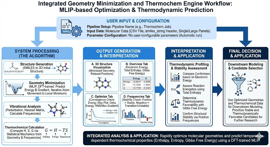
Revilico’s Geometry Minimization and Thermochem Engine rapidly minimizes molecular geometries and computes temperature-dependent thermochemical properties, enabling fast prediction of reaction energetics, conformational stability, and chemical feasibility without expensive quantum mechanical calculations. This engine is best used when you need to optimize molecular structures to their lowest-energy conformations and predict thermodynamic properties for understanding reaction thermodynamics and molecular stability. This engine is key to understanding the driving energetics of intrinsic compound conformations to compare against protein ligand interaction conformations. This elucidates the energetic penalties of shifting compound geometries in pockets of proteins to ensure that thermodynamically, your system makes sense.
How does this engine work? We first start with our SMILES string input which we then convert into a 3D molecular structure. We then feed this structure into a model that will predict the energy as well as the energy gradient, giving the engine an instruction for which direction to move atoms in order to reach the lowest possible energy state for that molecule. By slowly adjusting the coordinates and positioning of the atoms in space and continuously calculating energies, we can find local thermodynamic equilibriums.Here is how the model works. Typically when calculating the energetics of a molecule we will use force fields, where we will calculate the total bond energy by summing up energy from the bonds, angles, torsions, van der Waals, steric hinderance, and electrostatics. Traditional forcefields are fast, but they are more limited in accuracy. The more accurate way of doing this is by doing large scale Density Functional Theory (DFT) calculations, however doing this at scale is very computationally expensive. Traditionally, DFT has been used to help approximate the physical interactions and energetics of electrons within biochemical systems, and is a computationally feasible way to find approximate solutions to Schrodinger’s equations without unimaginable amounts of computation. DFT usually follows a general framework based on the following equation:[−21∇2+Vext(r)+VH(r)+VXC(r)]ψi(r)=ϵiψi(r)Where ψ(r) is Kohn_Shams orbital, -½ ∇² is the kinetic energy, V_ext(r) is the external potential, V_H(r) is Hartree term, and V_XC(r) is the exchange correlation. DFT has been a widely used solution to analyzing chemical systems at the quantum level, but recent breakthroughs and data collections with UMA/QMOL25 datasets by Fairchem also enable for the training of AI models on these datasets for increased speed and accuracy.This engine introduces a machine learned interatomics potential (MLIP) trained on large scale Density Functional Theory data (DFT) from the Fairchem team at Meta. This data comes from a quantum mechanical calculation that will model electron density, electronic energy, and nuclear forces at scale across chemical and protein systems. The data itself contains atomic numbers, 3D atomic coordinates, total electronic energy from DFT calculations, and atomic forces or the gradient of the DFT energy. The data will often contain multiple geometries of the same molecule so it is trained on many off-equilibrium geometries so it can learn how energy changes when atoms move. How the model works is that for each molecule, the model will receive the atomic identity, atomic position, and their local atomic environment (constructing a local neighborhood around each atom to see which atoms are nearby, their distances, and their relative orientation). The model will output the total energy which is an approximation to the DFT total electronic energy, and the negative gradient of the energy, which will show directionality for each atom to reach its lowest energy state and its eventual geometrically optimal position in 3D space with minimized energetics.At this point, the molecule is at a stable, low energy 3D conformation. We want to compute our thermochemistry step. Thermochemistry can be defined as studying how the heat energy changes during chemical reaction, with an emphasis on how the heat is absorbed or released. Essentially what we want to understand is how stable a molecule is, how it responds to temperature, and how favorable processes involving this molecule are. Thermochemistry is based on this equationG=H−TSWhere G is the Gibbs free energy or the balance between energy and disorder, H is enthalpy or how much internal energy the molecule has, S is entropy and how much freedom or disorder the molecule has and T is temperature.For measuring thermochemistry, the engine will capture the following properties. First, atomic masses, where heavier atoms move more slowly meaning lower vibrational frequencies. Second, molecular geometry, where this will define how atoms are connected and how rigid or flexible the structure is. Third, moments of inertia, which is derived from atomic masses and is their distance from the center of mass. This is required to compute rotational entropy. Fourth, potential energy surface curvature, where it will answer the question if we move the atoms away from this geometry, how quickly does the energy increase. This comes from the second derivatives of energy and is estimated using the MLIP from DFT calculations. Here steep curvatures mean stiff vibrations and low entropy. Lastly, molecular symmetry, where symmetry will affect rotational entropy.The main goal of this engine is to compute enthalpy and entropy. To calculate this we must understand how the molecules vibrate. To do this the engine will slightly perturb the atom positions. It will observe how the forces change, building a matrix describing how motion couples between atoms. Then it will diagonalize the matrix.Enthalpy is calculated with the following equation:H=Helec+Htrans+Hrot+HvibWhere:Helec≈EelecHtrans=23kTHrot=23kTHvib=i∑[2hνi+exp(hνi/kT)−1hνi]Entropy is calculated with the following equation:S=Strans+Srot+SvibWhere:Strans=k[ln(h3(2πmkT)3/2NV)+25]Srot=k[ln(σπ(h28π2kT)3/2IAIBIC)+23]Svib=ki∑[exp(hνi/kT)−1hνi/kT−ln(1−exp(−hνi/kT))]From there we have entropy and enthalpy terms. We will now be able to calculate our Gibbs Free Energy over different temperatures using this equationG=H−TS