FEP Engine - Revilico

Why Use this Engine?
In this document, we will use Revilico’s Free Energy Perturbation Engine to support lead optimization and structure activity relationship refinement by evaluating closely related compounds, and analyse its particular effects on binding in which docking itself cannot fully resolve. These methods differ from the MMPBSA/MMGBSA screens in that it runs alchemical transformations of the ligand before calculating free energies, whereas the MM(PB/GB)SA simulations run screenshot interpretations of free energy across a molecular dynamics trajectory.`

Background
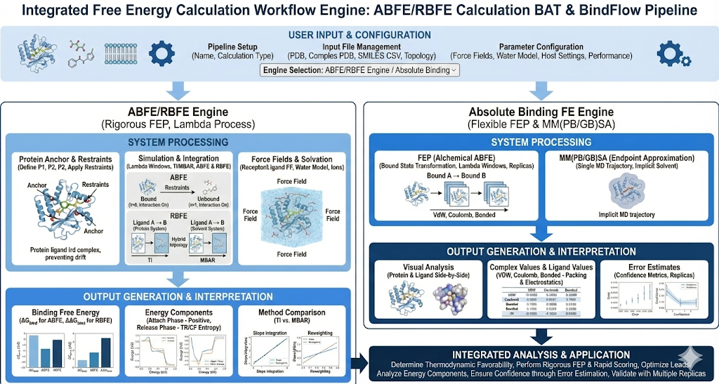
Before diving in, we need to understand what Free Energy Perturbation is. Free Energy Perturbation can be used to answer the two following questions with the two following methods. Absolute Binding Free Energy (ABFE) answers the question: How favorable is it for a ligand to bind to a protein? (i.e. if it is more favorable for the ligand to be in a bound state with the protein or an unbound state). We can think of it with this analogy. Sitting down in a chair (i.e. the bound state) is not the natural state (i.e. standing up), however it is preferred since it is the state in which we use less energy. Relative Binding Free Energy (RBFE) answers the following question: Does Ligand B bind better or worse than Ligand A to the same protein, and by how much? For ligands that are similar, docking has trouble finding differences in binding with high resolution .RBFE proposes a solution in which we will be able to differentiate between 2 or more very similar ligands for the purpose of lead optimization. It allows us to see whether a particular chemical modification improves or weakens binding relative to an existing ligand. Why is Free Energy Perturbation so important? For one, it measures thermodynamic favorability, not just pure binding events/interactions. It is not solely based on binding energetics but also loss of ligand flexibility, solvent displacement and reorganization, and protein ligand dynamics, taking into account the entire system of interest to find global minima of energy across protein, solvent, and ligands in different states. Secondly though it is quite computationally expensive, it is one of the most accurate computational tools available particularly for Lead Optimization - and it generally has the greatest experimental translation rates. We have 2 engines in our Free Energy Perturbation Suite: ABFE/RBFE Engine and the Absolute Binding FE. We can first begin with the ABFE/RBFE Engine engine . With ABFE, like we stated above, we are answering the question of whether it is more favorable to be in a bound or unbound state. To do this, we first have to resolve a system of a protein, ligand, solvent, ions, and restraints. Here we will apply a force field to every component of the system. To learn more about force fields, please refer to the Molecular Dynamics Documentation here). Revilico OS is also constantly updating it’s forcefields, and we are experimenting with classical forcefields as well as machine learning force fields (MLFFs, MLIPs, and NNPs). We will now introduce the concept of lambda windows. In our simulation, we essentially run molecular dynamics simulations across different snapshots of the simulation as we run different transformations of the ligand within what’s called ‘Lamba Windows’. We will first start with the ligand bound to the protein (interaction on) and over the course of the simulation’s lambda window snapshots, we transform the ligand to be fully unbound from protein (interaction off). To prevent the ligand from drifting off when the interaction is off, and so that we can correctly account for the loss and recovery of binding entropy, we introduce protein restraints, which will hold the ligand near binding site, fix its orientation relative to the protein, and prevent uncontrolled defusion. These are distance restraints, angle restraints, and dihedral restraints, and we also refer to them as anchors. Within the process of creating lambda windows, where we are taking MD screenshots at each window, we are going to measure what the energy cost is of going from a bound state to free state. If it costs a lot of energy for the ligand to be dissociated, or if there is favorable Gibbs Free Energy when binding, the ligand will prefer to be in a bound state, and this can be measured with dGbinding, also known as Binding Free energy, which is calculated with the following equation

\Delta G_{\text{bind}} = G_{\text{bound}} - G_{\text{unbound}}

Where negative delta G is favorable and positive is unfavorable. These are the thermodynamic drivers of binding interactions between ligands and proteins. We can now dive into Relative Binding Free Energy (RBFE). With RBFE we are answering the question: does ligand A bind better or worse than ligand B? To do this we have to define our two systems. Our first system is our ligand bound to protein state (ligand protein MD simulation) and our second system would be our ligand in our solvent state (ligand water MD simulation). In each system, a hybrid ligand topology is constructed in which shared atoms remain unchanged while ligand specific nonbonded interactions are smoothly scaled using an alchemical coupling parameter lambda (essentially changing our ligand from ligand A to ligand B over these lambda windows). An MD simulation is conducted at each lambda step, where we can calculate the RBFE values with the following equation

\Delta\Delta G_{\text{bind}} = \Delta G_{\text{bound}}^{A \to B} - \Delta G_{\text{solv}}^{A \to B}

We can now dive into our Absolute Binding FE Engine. Here we have 2 calculation types: FEP and MM(PB/GB)SA. Here we can first begin with FEP. With this calculation we are answering the question: if I modify this ligand into a new analog, does this new version interact more favorably with the target protein? The workflow behind this engine is very similar to that of the RBFE calculation engine as described above, with the exception that we are only interested in the bound state and not the solvent state, i.e. we are interested in:

\Delta G_{\text{bound}}^{A \to B}

With the MM(PB/GB)SA, we are answering the following equation: based on realistic protein ligand conformations, how energetically favorable does this ligand look when bound to the protein? What MMPBSA and MMGBSA does give is a relative binding strength estimate, which is useful for comparing compounds and identifying promising leads quickly. From a computational standpoint, MMPBSA and MMGBSA estimate an endpoint binding free energy using the following equation:

\Delta G_{\text{bind}} \approx \langle G_{\text{complex}} - (G_{\text{protein}} + G_{\text{ligand}}) \rangle

Where it is averaged over snapshots extracted from an MD trajectory, with solvent treated implicitly via Poisson–Boltzmann (PB) or Generalized Born (GB) models. What this essentially means is that we are simply running an MD simulation, calculating the binding free energy of the entire complex itself, the binding free energies of the protein without the ligand, and the ligand without the protein, to see whether it is more favorable to be bound or be unbound. This is different from our FEP simulations in the sense that we are not incorporating lambda windows and alchemical transformations to gradually simulate change, whether it be unbinding ligand from protein (ABFE) or morphing ligand A to ligand B (RBFE or FEP), and running MD simulations at each window. For MMPBSA and MMGBSA we are only running 1 MD simulation and running these calculations continuously as the system progresses over time. In our output we are presented with the 3D graphic of our Protein Ligand Complex on the left, on the top right presented with the Binding Free Energy value in kcal/mol, and on the top right presented with all the Energy Components metrics on the bottom left. For understanding the Binding Free Energy Metric. Binding Free Energy is derived from the following equation:

\Delta G_{\text{bind}} \approx \langle G_{\text{complex}} - (G_{\text{protein}} + G_{\text{ligand}}) \rangle

Where it represents the reversible works required to remove the ligand from the binding site into bulk solvent. For interpretation, Negative Delta G indicates binding is thermodynamically favorable, where more negative indicates stronger binding. For the attach phase, this is the free energy cost of applying restraints that fix the ligand position, orientation, and conformation, essentially this is the cost of ensuring that the ligand does not float away when we are in unbound state. For interpretations, these values will always be positive, and larger values mean that the ligand had more freedom before restraint. The part of this table is based on whether we choose Thermodynamic Integration (TI) or Multi State Bennett Application Ratio (MBAR). Downstream Interpretations The Thermodynamics Integration equation is a method for calculating binding free energy. Previously we introduced the concept of lambda windows. Rather than comparing absolute energies between windows, TI evaluates the change in energy with respect to lambda at each window and integrates these values to obtain the total free energy difference. The smoothness of this integration reflects how gradually and stably the system transitions between states. In other words, we are measuring how the system’s energy changes as interactions are weakened, and these changes are combined to determine the overall free energy. The Thermodynamic Integration equation is defined as follows:

\Delta G = \int_0^1 \left[ \frac{\partial U}{\partial \lambda} \right]_\lambda d\lambda

Where U is the system’s potential energy from the Hamiltonian force field, and ∂U/∂λ is the averaged local slope of the force field energy with respect to lambda, measured during MD at each lambda window and integrated to compute free energy. The Multistate Bennett Acceptance Ration (MBAR) is an additional method for estimating free energy differences across multiple simulation states. Instead of focusing on local changes between neighboring lambda windows like TI, MBAR analyzes all sampled configurations across all windows to determine the most probable free energy differences. It evaluates how well each molecular configuration sampled at one lambda state would be explained by every other lambda state. It essentially reweights all snapshots using information from the entire ensemble, allowing it to extract the free energy difference that is most consistent with the full dataset. In simple terms, it answers the question: given everything we observed across all simulations, what single free energy difference best explains all the data. It can be denoted with the following equation

f_i = -\ln \sum_{n=1}^N \frac{\exp(-u_i(x_n))}{\sum_{k=1}^K N_k \exp(f_k - u_k(x_n))}

Where ui(xn) is the reduced potential energy of configuration xn evaluated at lambda state i, ,and the solution yields free energy differences between states. These differences are then combined to produce the final binding or transformation energy. In the table we are measuring either TI or MBAR as it relates to electrostatics (charges interacting with protein and solvent) and Lennard-Jones (Shape complementarity, sterics, and dispersion). For Electrostatics we would want a value that is near zero or mildly positive or negative since large negatives will indicate artifacts. For Lennard Jones, we want a moderate magnitude that is well balanced with electrostatics. For the release phase, Release Ligand TR is the translational and rotational entropy which is the term that accounts for the freedom a ligand gains when it is no longer positionally and orientationally restrained. Release Ligand CF is conformational freedom, which measures the entropy gained when the ligand is allowed to flex internally again. These terms are meant to correct the binding energy for entropy lost during calculation since we have placed protein restraints. To interpret Release Lignad TR we are looking for a value that can cancel out our attach term. With Release Ligand CF larger magnitudes indicate more flexible ligands and smaller indicate rigid ligands.

Engines