Documentation Index
Fetch the complete documentation index at: https://docs.revilico.bio/llms.txt
Use this file to discover all available pages before exploring further.
Why Use this product?
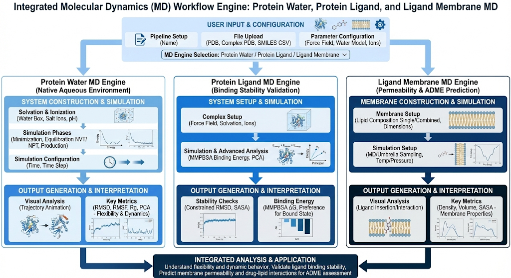
Molecular Dynamics (MD) simulations reveal how biomolecular systems evolve over time in their native environments, capturing the dynamic behavior that static structures miss, from protein flexibility and binding site breathing (protein-water), to ligand binding stability and key interaction identification (protein-ligand), to membrane permeability and drug-lipid interactions (ligand-membrane). These simulations bridge the gap between static docking predictions and experimental validation, helping drug discovery teams prioritize compounds by assessing binding pose stability, understanding target flexibility, and predicting ADME properties like membrane permeability. By providing atomic-level insight into molecular motion and interactions over nanosecond-to-microsecond timescales, MD enables structure-based drug design to move from static snapshots into dynamic, physically realistic predictions.
Background
Proteins, ligands and membranes are dynamic systems that continuously fluctuate, reorganize, and respond to their environment. Where tools like Docking cannot capture this system and can only capture static snapshots of these interactions, Molecular Dynamics (MD) proves to be a solution by providing a physics based framework for understanding how biomolecular systems behave over time. Now what does Molecular Dynamics actually do? At its core, MD simulates how atoms move as a function of time by applying classical mechanics. Generally MD follows this corresponding pipeline. First system construction places (proteins, ligands, and/or lipids) in a periodic simulation box, typically solvated with explicit water molecules and ions to mimic physiological conditions. Second we assign a force field. These are the parameters assigned to each atom (i.e. partial charge, bonded connectivity, nonbonded interaction parameters, etc.). Our third step is energy minimization. This step removes steric clashes or unrealistic geometries that could cause numerical instability. Our next step is bringing the system to equilibration, both to a target temperature and allowing the system density and box dimension equilibrate to realistic pressure. The next step is production molecular dynamics where the system is simulated over time, generating a trajectory that captures atomic motion under realistic conditions.
Now we can dive into the theory. The behavior of our system is governed by a classical potential energy function or the force file which is expressed with the following equation.
E=∑interactions
Etotal=Ebonds+Eangle+Edihedral+EVDW+Eelec
Ebond=∑kb(r−r0)2
Eangle=∑k0(θ−θ0)2
Edihedral=∑2Vn(1+cos(nϕ−γ))
EVDW=∑4ϵ[(rσ)12−(rσ)6]
Eelec=∑(qi×qj)/(4πϵ0rij)
From the Etotal function, forces acting on each atom are computed as
Fi=−∇riE
Using Newton’s equation F = ma, we are then able to use this calculated force and the mass of each atom to update positions over time by updating our velocity that results from acceleration from this equation.
With temperature in MD, it represents the average kinetic energy of atoms. Initial velocities are drawn from a Maxwell-Boltzmann distribution, and thermostats are used to maintain the desired temperature statistically over time. .Thermal motion ensures that atoms continuously explore conformational space, allowing the system to sample biologically relevant states rather than freezing into a single configuration
Running Snapshot/Post-Processing Free Energy Methods
For MMPBSA, we are evaluating whether is it preferred for the ligand to be docked in the protein or if it is energetically favorable for the ligand to be free. In order to calculate MMPBSA we do the following: 1) we take note that we have our entire MD simulation made up of all the snapshots based on our intervals across the total simulation time.. We will remove the early snapshots as this is the equilibration step and therefore are not representative samples for calculating energies, and ensure that our calculation does not include extreme values that can heavily skew our outcomes. From there, we take the snapshots at the defined intervals and we calculate the following equation at each time step and average out all the values across each snapshot/interval.
ΔGbind=Gcomplex−(Gprotein+Gligand)
G≈EMM+Gsolv
Where EMM is the forcefield equation defined above as Etotal Or ΔGbind. When we decompose this equation, essentially we will need to compute the energetics using our selected force fields for the entire complex (protein with ligand docked), the energies of the force fields of the protein on its own (internal forces of the protein atoms acting upon itself), and the force field of the ligand on its own (forces of the ligand atoms acting upon itself). Furthermore we can decompose Gsolv to the following equation:
Gsolv=GpolarPB+GnonpolarSA
Where GpolarPB is the electrostatic cost of putting a charged molecule in water and GnonpolarSA is the hydrophobic cost of creating a cavity in water. Essentially what we are calculating is the free energy cost of whether the ligand is better in the bound position or whether it is better unbound. How we can interpret this is that very low delta G_total values indicate strong preference for the bound state which is the preferred value when it comes to evaluating whether a compound is a strong candidate. These energetic calculations elucidate a more sophisticated binding composition, breaking down all of the energetic contributions to direct ligand protein engagements.
Interactive Results Viewer
Explore Protein-Ligand MD simulation results interactively. View trajectory analysis, RMSD plots, energy decomposition, and MMGBSA binding free energy contributions.