Docking Engine - Revilico

Why use this engine?

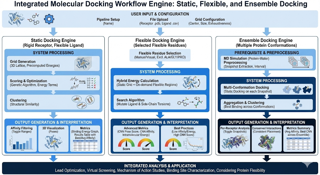
In this document we will use Revilico’s Virtual Screening Engine to dock a library of candidate ligands against a protein target in order to identify the most promising compounds for downstream analysis.. We begin with rigid docking to enable high-throughput screening and rapid downselection. Selected ligands are then evaluated using flexible docking,, which allows key protein residues to move and capture more realistic ligand-protein interactions.. Finally, ensemble docking is applied to assess ligand binding across multiple protein molecular dynamic conformations, providing insight into how ligands interact with the dynamic nature of the protein Docking Engine

Background

Molecular docking is critical in chemistry for predicting the most stable, 3D orientation of a ligand within a protein binding sight along with it’s energetics and binding affinities, directly informing rational drug design, virtual screening, and understanding molecular drivers of binding. Running physical assays is a task that can be both expensive and very time consuming. Without computational tools such as docking, chemists would have to send incredibly large compound libraries into high throughput screening facilities in order to get a few hit compounds that effectively bind to the protein. Docking is an effective solution where chemists will be able to downselect their compound libraries to a much smaller batch of compounds with high predicted affinities, essentially cutting down on both time and cost to run experimental validation. In our own internal studies, we have observed almost a 20x improvement of our high throughput screening hit rates when utilizing these engines. We introduce Revilico’s Virtual Screening Engine, an engine composed of 3 different types of docking: Static Docking, Flexible Docking, and Ensemble Docking. Static Docking In static docking, we will predict ligand binding modes and relative affinities with a validated binding site using a fixed protein structure (e.g. the protein remains rigid whereas the ligand is flexible and can explore different poses). Static Docking is utilized for high throughput screens of larger libraries (>2M compounds). Overall, it is a GPU accelerated algorithm that allows for us to calculate binding scores and conformations of compounds at scale to better analyze vast chemical spaces without needing to run computationally extensive algorithms. Before diving into how static docking works, we need to understand how we can calculate binding energy. It can be calculated with the following equation, composed of several summed energetic components at the atomistic level:

E_{\text{binding}} = E_{\text{vdW}} + E_{\text{elec}} + E_{\text{hbond}} + E_{\text{desolv}} + E_{\text{tors}}

E_{\text{vdW}}

is energy from Van der Waals calculated with the following equation

E_{\text{vdW}} = \sum \left( \frac{A}{r^{12}} - \frac{B}{r^{6}} \right) \cdot S(r)

Where A,B are Lennard-Jones parameters (atom-type specific), r is interatomic distance, and S(r) is a smoothing function.

E_{\text{elec}}

is the energy from electrostatics calculated with the following equation

E_{\text{elec}} = \sum_{i<j} \frac{1}{4\pi \epsilon_0} \frac{q_i q_j}{\epsilon(r_{ij}) r_{ij}}

Where

q_i

, and

q_j

are partial atomic charges, epsilon(r) is distance-dependent dielectric, and r is interatomic distance

E_{\text{hbond}}

is energy from hydrogen bonding calculated with the following equation:

E_{\text{hbond}} = \sum \left( \frac{C}{r^{12}} - \frac{D}{r^{10}} \right) \cdot \cos(\theta)

Where C, D are H-bond parameters (donor-acceptor specific), r is donor-acceptor distance, theta is angle deviation from ideal geometry

E_{\text{desolv}}

is energy from desolvation calculated with the following equation:

E_{\text{desolv}} = \sum_{i \in \text{ligand}} \sum_{j \in \text{ligand}} (S_i V_j + S_j V_i) \exp\left(-\frac{r_{ij}^2}{2\sigma^2}\right)

Where S_i is solvation parameter of atom i, V_j is volume of atom j, sigma (σ) is a Gaussian decay constant, and r is interatomic distance.

E_{\text{tors}}

is torsional energy defined by the following equation:

E_{\text{tors}} = N_{\text{tors}} \cdot W_{\text{tors}}

Where N_tors is the number of rotatable bonds in ligand and W_tors is the torsional penalty weight. Where N_tors is the number of rotatable bonds in ligand and W_tors is the torsional penalty weight. The first step of static docking is parameterization, where we take our input protein structure and assign atom types, and calculate partial charges. We then have our grid, which is the only space in which our ligand can be located throughout the duration of the calculations. This grid is synonymous with the structure of a 3D lattice. At each atomic position within this grid we calculate the binding energies of each type of atom-atom interaction to get a total binding affinity score or kcal/mol energy term. So for all points in the grid we would map the interaction energy defined by E_binding of all possible atomic configurations of the ligand. We now have a matrix with all of our mapping functions for all the possible atom types and conformational configurations. We now will seed thousands of random configurations of the ligand poses. With this we can score based on E_binding and can have a general landscape of what particular poses we think will be successful in binding. The next step is to take a number of these poses with relatively good E_binding and optimize them. We then will introduce a genetic algorithm, which will essentially mutate these optimized poses with other poses that have better, more optimized scores based on the scoring function of the algorithm. We will then repeat this process over and over again. Now, at this point, we have several optimized poses solely based on binding scores. However docking is not solely based on binding energy it is also based on the geometry of the poses. We then introduce a clustering algorithm where we take the best pose based on binding energy and cluster similar poses based on structural resemblance. We now have clusters of several poses based on different geometries. We then take the best proposed binding score from each cluster and report that in our docking results. Usually, there will be around 9 of the top poses that are reported into our downstream analytics page. Flexible Docking The flexible docking algorithm is the secondary step for large scale screens and can usually be used for re-scoring your filtered batch of molecules from static docking that you retrieved and filtered. Traditionally, after receiving the results of the static docking you can filter based on chemical space analysis and diversity along with binding affinity predictions. Usually, you want to maintain a large enough batch for re-scoring as static docking is notoriously going to have a higher rate of false positives and negatives as it is optimized for speed, and not so much refined accuracy. Flexible docking will operate in two distinct phases: pose sampling and pose ranking. The algorithm works by combining empirical physics based equations with CNN rescoring to optimize the poses for physical feasibility and reduced steric clashes. The CNN engine provides a pseudo affinity score in the form of a pK range along with more physically relevant pose predictions. During the conformational search phase, we will use the following function to guide pose optimization:

E_{\text{sampling}} = \sum \left[ w_1 e^{-\left(\frac{r_{ij}}{\sigma_1}\right)^2} + w_2 e^{-\left(\frac{r_{ij}}{\sigma_2}\right)^2} + w_3 f_{\text{repulsion}}(r_{ij}) + w_4 f_{\text{hydrophobic}}(r_{ij}) + w_5 f_{\text{hbond}}(r_{ij}) \right] + w_6 N_{\text{rot}}

Where Two Gaussian terms model smooth distance dependent attraction at different distance ranges. The first narrow Gaussian captures short range attractive interactions such as hydrogen bonding and close van der waals contacts while the second broad gaussian captures longer range dispersion-like attractions. The weights w1 and w2 are empirically fitted to reproduce experimental binding affinity scores between protein and ligand f_repulsion models the steric clashes, f_hydrophobic approximates burial effects, f_bond captures directional hydrogen bonding, and N_rot applies a linear penalty for ligand rotatable bond. The search operates on both ligand conformation space and optionally on selected protein side-chain residues that you tag in the parameter section. These flexible residues gain rotational freedom while maintaining fixed atom types, charges, and bond lengths. The static portions of the protein retain the precomputed grid-based energy maps from static docking, while flexible regions are computed on-demand during the search. Usually, flexible residues are selected based on already known co-crystal structures that reveal key amino acids for biological activity or binding. After generating candidate poses through our sampling step above, we apply a fundamentally different scoring approach using convolutional neural networks (CNN). Our scoring will then combine the scores of both our sampling component and our ranking component shown with the following equation

E_{\text{flex}} = \alpha E_{\text{sampling}} + \beta S_{\text{CNN}}

In practice, the CNN score (beta) dominates the final ranking, with the physics/sampling score (alpha) serving primarily as a regularizer to keep poses physically reasonable. The CNN has learned statistical patterns of what binding looks like from experimental structures rather than computing physical binding energies. For Flexible docking we will capture the following metrics: Best Affinity, Best Intramol, Best CNN Pose Score, and Best CNN Affinity. Best Affinity is the additive, empirical energy calculations where lower energy indicates more thermodynamic favorable interaction. It can be denoted by the following equation:

\Delta G = \sum_{i \in \text{ligand}} \sum_{j \in \text{protein}} \left[ w_1 f_{\text{gauss1}}(r_{ij}) + w_2 f_{\text{gauss2}}(r_{ij}) + w_3 f_{\text{repulsion}}(r_{ij}) + w_4 f_{\text{hydrophobic}}(r_{ij}) + w_5 f_{\text{hbond}}(r_{ij}) \right] + w_6 N_{\text{rot}}

Where the summation is over rigid pairs, combining van der Walls, Lennard-Jones, repulsion, electrostatic, and desolvation terms, plus a rotational entropy penalty. Best Intramol is the minimum intramolecular energy of the ligand, where its role is to filter out physically implausible strains. Higher values often mean steric clashes. It can be denoted by the following equation

E_{\text{intra}} = E_{\text{vdW}} + E_{\text{repulsion}} + E_{\text{torsion}}

Best CNN Pose Score is a binary metric for protein-ligand geometry/poses and physical realism. Scores range from 0 to 1 where 1 indicates the highest score. It can be denoted by the following equation: Best CNN Pose Score =

\max_{p \in P}(\text{good pose} \mid p)

Where the classifier model is trained on native crystal structures and decoys. Best CNN Affinity is the output of a supervised regression model that maps 3D conformation to a binding strength proxy. This is a pK value, therefore higher values indicate higher affinity. It can be denoted by the following equation:

\hat{y} = f_{\theta}(X)

Where X is the voxelized 3D representation of a docket pose, fθ is the deep 3D convolutional neural network, and y_hat is the predicted binding affinity Ensemble Docking With Ensemble Docking we introduce Molecular Dynamics as a precursor and pre-processing step of the protein target of interest before moving into Flexible Docking scoring. How this works is that we will run a Protein Water MD simulation which will simulate a single protein in a solvent environment without any ligand present, allowing the protein to explore its natural conformations over time under physically realistic conditions. To learn more about Protein Water MD please refer to the documentation here. What we will do is we have a simulation that lasts a certain amount of time ( in nanoseconds). We will then extract screenshots of the protein at different time intervals. At these time intervals within the simulation, we will extract snapshots of the protein ‘trajectory’ to further be processed and structurally prepared for scoring and then we will perform flexible docking as described above for each snapshot. Now we will have several different protein poses for every ligand being tested across all these snapshots. This is an intermediary tradeoff where we get the nuance of a changing protein structure, mixed with the speed of our docking engines. After collecting all of the data, we then aggregate all of the different combinations of compounds with the different protein structures/models to get a collective picture of more realistic ligand protein binding affinity measures. . The next step would then be to cluster the poses based on structural similarity. For this clustering process, it is done after conformational sampling of poses of ligands within singular protein structure snapshots, rather than clustering and aggregating across all snapshots. This interpretation will focus on recurring binding patterns, conserved interactions, and consistent ligand placement relative to key residues, analyzed during more dynamic conditions.

Interactive Results Viewer

Explore molecular docking results interactively. View receptor-ligand 3D structures with pose selection, binding affinity charts, and RMSD analysis.

Engines

​Why use this engine?

​Background

​Interactive Results Viewer

Why use this engine?

Background

Interactive Results Viewer