RevTorsion

​

Why Use This Engine?

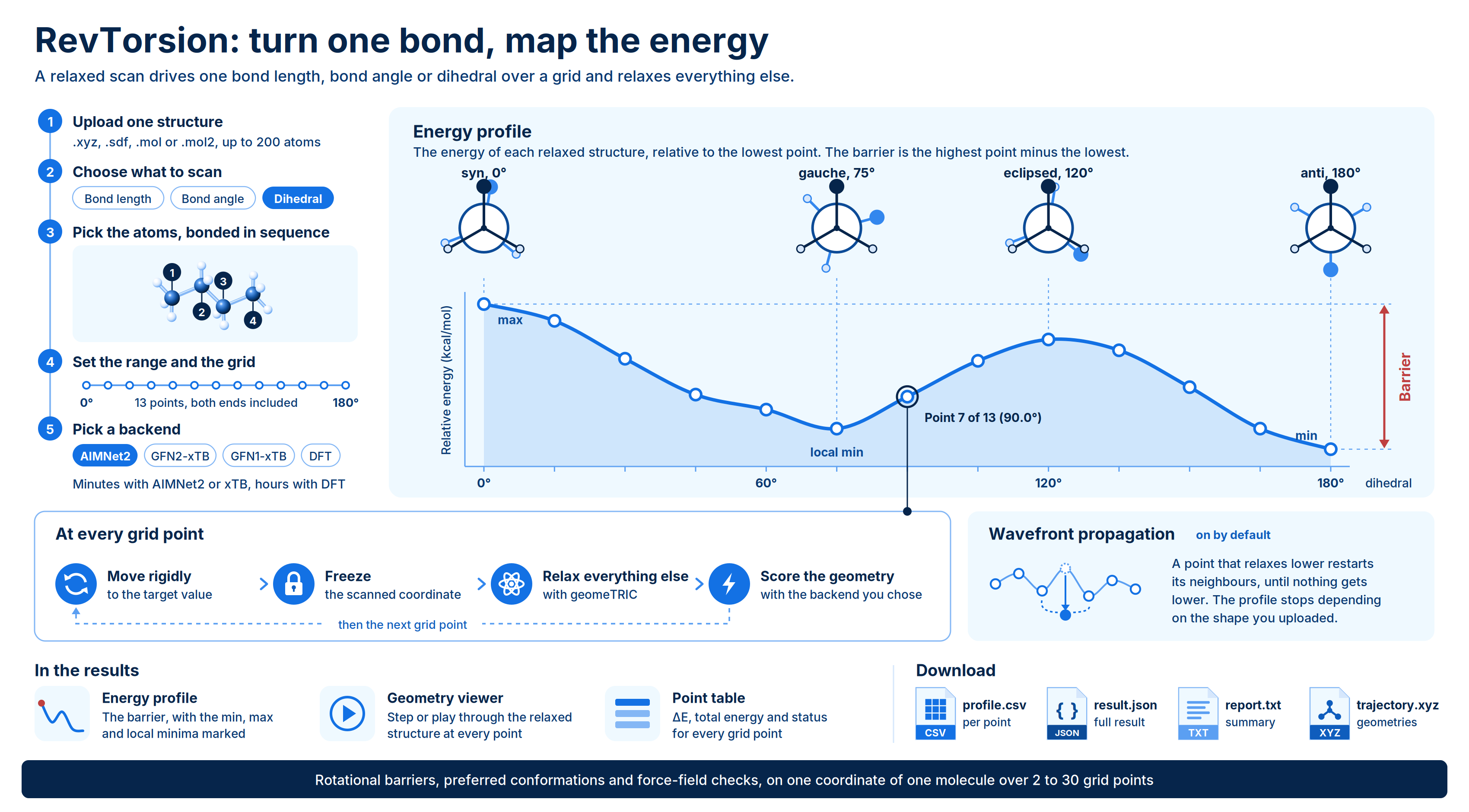
RevTorsion runs a relaxed scan. It drives one internal coordinate of a molecule (a bond length, a bond angle or a dihedral) through a series of fixed values. At each value it relaxes the rest of the structure with a constrained geometry optimization. The result is an energy profile along that coordinate, with the minimum, maximum, rotational barrier and a relaxed geometry at every grid point. Use RevTorsion when you need to know how the energy of a molecule changes as one part of it moves. Typical uses:

• Measure rotational barriers. Scan the dihedral around an amide, urea, biaryl or other rotatable bond to see how freely it turns and which conformations are preferred.
• Find preferred conformations. Locate the global minimum and any local minima along a torsion, for example to check whether a docked or designed pose sits in a low-energy region.
• Parameterize or check force fields. Compare a quantum-level torsion profile against the one your force field produces.
• Probe bond stretching and angle bending. Scan a bond length or bond angle to see how stiff it is, or to follow a bond as it lengthens.

Each run scans one coordinate of one molecule, over 2 to 30 grid points. You can choose a neural network potential (AIMNet2), semiempirical tight-binding (GFN2-xTB or GFN1-xTB) or density functional theory (DFT) to compute the energies.

​

Background

A rigid scan changes one coordinate and leaves every other atom where it was. A relaxed scan, which is what RevTorsion runs, holds the scanned coordinate $q$ at each target value $q_k$ and lets every other degree of freedom relax: $$E(q_k) = \min_{\mathbf{R}} \; E(\mathbf{R}) \quad \text{subject to} \quad q(\mathbf{R}) = q_k$$ where $\mathbf{R}$ is the set of atomic positions. A relaxed profile is lower than a rigid one and reflects what the molecule actually does as the coordinate changes. The grid. The grid includes both ends. With num points from start to stop, the spacing is $$\Delta q = \frac{\text{stop} - \text{start}}{\text{num} - 1}$$ so a dihedral scan from 0° to 180° with 7 points visits 0°, 30°, 60°, 90°, 120°, 150° and 180°. Bond lengths are in ångström (Å) and angles and dihedrals in degrees (°). Each grid point. RevTorsion first moves the molecule rigidly so the scanned coordinate sits exactly at the target value. For a dihedral, this rotates the whole group of atoms on one side of the central bond. It then freezes that coordinate and optimizes everything else with the geomeTRIC optimizer. Because the geometry is moved rigidly, the atoms you pick must be bonded to each other in sequence, and the bond being turned cannot be part of a ring. Wavefront propagation. In a simple scan, every point starts from your input structure. Wherever that starting geometry falls into a different energy basin, the profile jumps and can show a barrier that isn’t real. RevTorsion avoids this with wavefront propagation (Qiu et al., J. Chem. Phys. 2020, the method used in torsiondrive). Whenever a grid point relaxes to a lower energy than it had before, RevTorsion uses that geometry to re-start the neighboring grid points. Improvements spread outward until nothing gets lower. This takes roughly twice as many optimizations, and the resulting profile no longer depends on the conformation you uploaded. Relative energies and the barrier. Each point’s energy is reported relative to the lowest point on the scan: $$\Delta E_k = \left( E_k - E_{\text{min}} \right) \times 627.509 \ \text{kcal/mol per Hartree}$$ The barrier is the highest point on the scan minus the lowest. A local minimum is an interior grid point that is lower than both of its neighbors, other than the global minimum. Choosing a backend. The backend is the method that computes the energy and forces at each geometry:

• AIMNet2 (ωB97M-D3) is a neural network potential trained on ωB97M-D3 DFT data. It is fast and, for the organic molecules it covers, more accurate than the semiempirical methods. It supports 14 elements (H, B, C, N, O, F, Si, P, S, Cl, As, Se, Br, I) and closed-shell molecules only.
• GFN2-xTB is a semiempirical tight-binding method that covers hydrogen through radon, including transition metals, and supports open-shell molecules. Use it when your molecule has an element AIMNet2 doesn’t cover or has unpaired electrons.
• GFN1-xTB is the older xTB parameterization. Prefer GFN2-xTB unless you are comparing against GFN1 results.
• DFT runs r²SCAN-D4 (a meta-GGA functional) or ωB97M-D3BJ (a range-separated hybrid) on a GPU. It gives reference-quality profiles but takes hours rather than minutes.

​

Validation

Against a published reference scan. RevTorsion was benchmarked against a published third-party AIMNet2 scan of a 27-atom phenyl-pyridyl urea (C₁₂H₁₁N₃O). The scan drove dihedral 9-8-10-23 from 0° to 180° in 30 points, with the Standard optimizer mode: The per-point difference comes from the AIMNet2 model weights, not from the scan. The reference used the original 2024 AIMNet2 release, while RevTorsion uses the current release. Running RevTorsion with and without wavefront propagation gave profiles that agree with each other to 0.02 kcal/mol while both differ from the reference by the same 0.53 kcal/mol. Across backends. Hydrogen peroxide’s O-O torsion, 7 points from 0° to 180°, with wavefront propagation on and def2-SVP for the two DFT functionals. Relative energies in kcal/mol: The two DFT functionals agree to within 0.23 kcal/mol over the whole profile. AIMNet2 agrees with ωB97M-D3BJ (the method it was trained on) to 0.13 kcal/mol near the minimum but underestimates the cis barrier by 1.87 kcal/mol (about 23%). Part of that gap may come from the small def2-SVP basis rather than the network. GFN2-xTB gets the shape wrong and puts the minimum at 180°.

​

Running the Engine

Open Quantum Chemistry > RevQuant > RevTorsion. The page has two tabs: Scan to set up a run and Analysis to view results.

​

Inputs

​

Preparing the input file

A scan needs real 3D coordinates, and it runs on exactly one structure because the scan is defined by atom numbers in that structure. SMILES input is not accepted.

• XYZ. Used exactly as given. Set the Charge and Spin multiplicity under Advanced, because an XYZ file doesn’t carry them.
• SDF, MOL or MOL2. Explicit hydrogens are kept. An SDF must contain only one molecule; a file with several is refused. A file with no 3D coordinates is refused. If you leave Charge at 0, the formal charge from the file is used.

To scan several molecules, or several coordinates of the same molecule, submit one run for each.

​

Full rotations

A dihedral grid wraps around only when it covers a full turn without repeating an end: the range plus one grid step must equal 360°. For example, 0° to 348° in 30 points (12° spacing) wraps, so 348° and 0° are treated as neighbors. A grid from −180° to 180° visits the same geometry twice, and a grid from 0° to 180° does not wrap.

​

Extra constraints

Under Advanced > Extra constraints, click Add to hold another coordinate fixed for the whole scan. For each constraint, choose the Coordinate, type the atom numbers, and enter a Value in Å or degrees. Leave Value blank to freeze the coordinate at whatever value it has in your input structure. Click the X to remove a constraint.

​

Optimizer modes

The optimizer mode sets how tightly each constrained optimization must converge. Every point is limited to 250 optimizer steps.

​

Run time and credits

Run time grows with the number of grid points, the size of the molecule and the backend, and roughly doubles with wavefront propagation on. As a guide for a 30-point scan of a 27-atom molecule with wavefront propagation on: The estimate shown after you submit is a guide, not a quote. DFT runs. DFT scans run on a GPU queue, which may take a few minutes to start. DFT cost grows roughly with the square of the number of basis functions, so molecule size matters more than the number of grid points. When you select DFT and upload a structure, the form shows an Estimated runtime. A DFT job has an 8-hour limit. If the estimate is over that limit, the form won’t submit and suggests ways to bring it down: turn off wavefront propagation, use fewer grid points, switch to r²SCAN-D4 (the cheaper functional), or use a faster backend. The estimate assumes def2-SVP. Credits. RevTorsion bills 1 credit per minute of runtime while the scan runs, starting with a charge when the scan begins. Time spent waiting in the queue is not billed. At that rate, a 5-hour DFT scan uses about 300 credits.

• Runtime Limit (Credits) is optional. Leave it blank to let the scan run to completion with no cap. If you set it, the scan stops when it reaches that many credits and the run ends with the status terminated_budget_exceeded.
• You need enough credits to start a run: at least your runtime limit, or 10 credits if you leave it blank. A run also stops if your credits run out.

​

Viewing Results

Open the Analysis tab and click a scan in the list. You can search the list by name, ID or status. Runs that are still in progress refresh automatically every 10 seconds. Click Change Scan to go back to the list.

​

Run statuses

A run can finish as processed with some grid points missing. The header then shows a partial badge, and the missing points appear as gaps in the chart and the table.

​

Results

The run header shows the coordinate type, how many points completed (for example 28 of 30 points completed), a partial badge when points are missing, and the total run time in seconds. Energy profile. A line chart of relative energy (kcal/mol) against the scanned coordinate (Å or degrees). Above the chart, the Barrier badge gives the highest point minus the lowest, in kcal/mol, along with a count of missing points. Markers label the min (global minimum), max and any local min. A missing point is drawn as a dashed line labeled gap, never as a zero. Hover over a point to see its value, relative energy, absolute energy in Hartree, and whether its optimization converged. Click a point to show its geometry. Geometry viewer. An interactive 3D view of the relaxed structure at the selected point, titled with its position and value, for example Point 3 of 15 (25.7°). Click the play button to animate the whole scan, or use the arrows and slider to step through points. Click XYZ to download the current frame. Point table. One row per grid point: Click a row to select that point in the chart and viewer.

​

Downloads

Click Download in the run header to open four files:

• profile.csv: one row per grid point, in grid order, with failed points kept as rows. Columns: index (numbered from 0), coordinate_angstrom or coordinate_degree, energy_hartree, relative_energy_kcal_per_mol, seed_energy_hartree (energy of the rigidly moved starting geometry), relaxation_hartree (how far the energy fell during optimization), optimizer_steps, optimizations (more than 1 means wavefront propagation re-optimized the point), converged, constraint_deviation_angstrom or constraint_deviation_degree (largest difference between the target and final value), and error.
• result.json: the full result document, with the scan request and settings, every point’s energies, geometry and diagnostics, the located minimum, maximum, local minima and barrier, the backend used, and timing.
• report.txt: a plain-text summary with the molecule, scan definition, method, a profile table, the extrema and barrier, convergence (how closely the coordinate was held and which points did not converge), and cost (optimizations, gradient evaluations and timing).
• trajectory.xyz: every relaxed geometry as one multi-frame XYZ file, one frame per completed grid point, for viewing or animating in other software.

The XYZ button in the geometry viewer downloads a single frame as point_NN.xyz, where NN is the grid index counted from 0.

​

Limits

• One molecule per run, up to 200 atoms and 10 MB. SMILES input is not accepted; the structure needs 3D coordinates.
• One coordinate per scan (a one-dimensional scan), with 2 to 30 grid points.
• The scanned atoms must be bonded in sequence, and a bond inside a ring can’t be scanned.
• Up to 10 extra constraints.
• AIMNet2 supports only H, B, C, N, O, F, Si, P, S, Cl, As, Se, Br and I, and closed-shell molecules only. GFN2-xTB and GFN1-xTB cover hydrogen through radon. DFT covers the elements of the def2-SVP basis set, which excludes the lanthanides cerium through lutetium.
• DFT scans must be estimated to finish within the 8-hour job limit.
• Absolute energies aren’t comparable between backends, or with other software. Compare relative energies (ΔE) and barriers instead.
• For an unconstrained geometry optimization, use RevGeometry. For a single-point calculation at a fixed geometry, use RevEnergy.