RevFukui

​

Why Use This Engine?

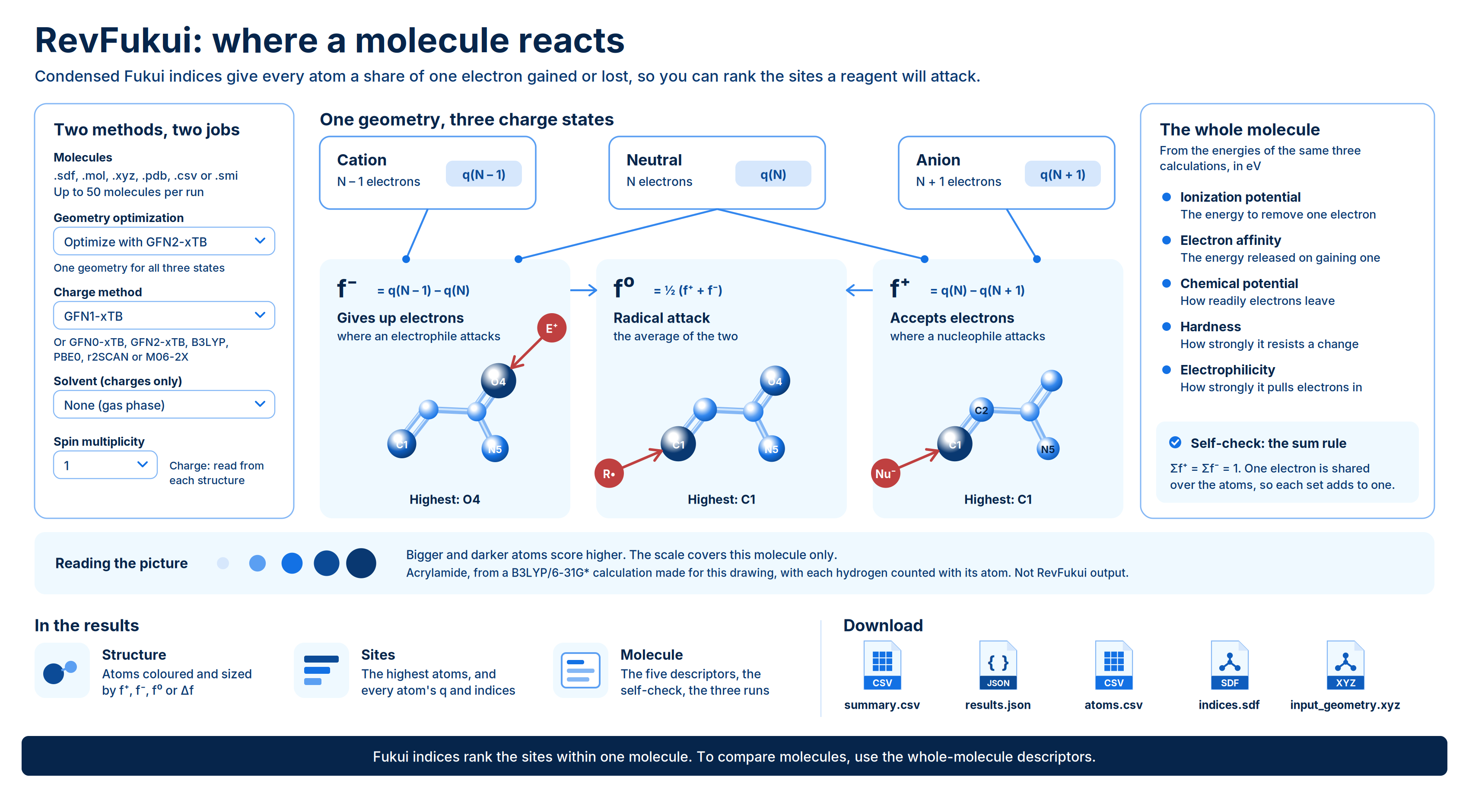
RevFukui tells you where a molecule reacts. It computes condensed Fukui indices, one number per atom, that show how the electron density at each atom changes when the molecule gains or loses an electron. The atoms with the highest values are the likely sites of attack by an electron-rich partner, an electron-poor partner, or a radical. Alongside the per-atom indices, RevFukui reports molecule-wide descriptors: ionization potential, electron affinity, chemical potential, hardness and electrophilicity. Typical uses:

• Find metabolic soft spots. Atoms that readily give up electrons are candidates for oxidative attack.
• Flag covalent and reactive liabilities. Atoms that readily accept electrons show where a nucleophile, such as a cysteine thiol, would attack.
• Predict regioselectivity. Compare the indices on candidate positions of a ring or scaffold to see which one a reagent prefers.
• Rank a series by overall reactivity. Compare electrophilicity and hardness across analogs.

You can submit up to 50 molecules in one run, as SMILES or as 3D structure files.

​

Background

The Fukui function describes how the electron density $\rho(\mathbf{r})$ of a molecule responds to a change in its number of electrons $N$ at a fixed nuclear geometry: $$f(\mathbf{r}) = \left( \frac{\partial \rho(\mathbf{r})}{\partial N} \right)_{v(\mathbf{r})}$$ In practice the derivative is replaced by finite differences between three calculations on the same geometry: the neutral molecule ($N$ electrons), its anion ($N+1$) and its cation ($N-1$). Condensing the density onto atoms with atomic charges $q_k$ gives one value per atom $k$: $$f_k^{+} = q_k(N) - q_k(N+1) \qquad f_k^{-} = q_k(N-1) - q_k(N) \qquad f_k^{0} = \tfrac{1}{2}\left(f_k^{+} + f_k^{-}\right)$$

• $f^{+}$ (accepts electrons) is where density arrives when the molecule gains an electron. High values mark sites of nucleophilic attack: the atoms an electron-rich partner goes for.
• $f^{-}$ (gives up electrons) is where density leaves when the molecule loses an electron. High values mark sites of electrophilic attack: the atoms an electron-hungry partner goes for.
• $f^{0}$ (radical attack) is the average of the two. High values mark sites a radical is likely to attack.
• $\Delta f$ (dual descriptor) combines the two into one signed number per atom:

$$\Delta f_k = f_k^{+} - f_k^{-}$$ A positive $\Delta f$ means the atom would rather accept an electron; a negative value means it would rather give one up. The indices are in electrons. Because the three calculations differ by exactly one electron, the indices over all atoms must each sum to one: $$\sum_k f_k^{+} = \sum_k f_k^{-} = 1$$ RevFukui checks this sum rule for every molecule and reports it. A molecule that fails the check had its charge states set up wrongly, and its numbers should not be used. The energies of the same three calculations give the molecule-wide descriptors:

• Ionization potential is the energy needed to remove one electron, from the cation and neutral energies.
• Electron affinity is the energy released when the molecule takes on one electron, from the neutral and anion energies.
• Chemical potential measures how readily electrons leave the molecule at all. More negative means they are held more tightly.
• Hardness measures how strongly the molecule resists a change in its electron count. A large value means it reacts reluctantly.
• Electrophilicity measures how strongly the molecule as a whole pulls electrons in. A large value means a strong electron acceptor.

Fukui indices distribute a fraction of one electron over the atoms of one molecule, so they rank sites within a molecule. Use the global descriptors, not the per-atom indices, to compare reactivity between molecules.

​

Two methods, two jobs

A RevFukui run has two separate method choices:

• Geometry optimization relaxes each structure once, in the gas phase, before the three calculations. The geometry only needs to be reasonable, so a fast semiempirical method is enough.
• Charge method runs the neutral, cation and anion calculations whose atomic charges and energies every reported number is built from. This is the choice that matters most.

The charge method can be a semiempirical tight-binding method (GFN0-xTB, GFN1-xTB or GFN2-xTB) or a DFT functional (B3LYP, PBE0, r2SCAN or M06-2X). DFT charge calculations use the def2-SVP basis set with no dispersion correction. Dispersion does not change atomic charges and cancels in the energy differences behind the global descriptors. RevFukui writes the level of theory in the shorthand charges//geometry. For example, the default is GFN1-xTB//GFN2-xTB: GFN1-xTB charges on a GFN2-xTB geometry. A DFT charge method adds the basis set, as in B3LYP/def2-svp//GFN2-xTB, and a solvent adds its model, as in GFN1-xTB/ALPB(water)//GFN2-xTB.

​

Running the Engine

Open Quantum Chemistry > RevQuant > RevFukui. The page has two tabs: Fukui to set up a run and Analysis to view results.

​

Inputs

Solvent. The solvent applies to the three charge calculations only; the geometry optimization is always in the gas phase. RevFukui picks the solvation model from the charge method: ALPB for the xTB methods and CPCM for the DFT methods. Both act inside the calculation, so the charges, and every index built from them, reflect the solvent. Charge and multiplicity. Leave Charge blank when a run mixes neutral molecules with ions, so each molecule keeps its own charge. XYZ files do not state a charge, so set it here for them. If the electron count makes the chosen Spin multiplicity impossible, RevFukui uses the nearest valid value and notes it on the molecule’s result.

​

Preparing input files

SMILES (.csv or .smi). A CSV holds a header row plus one row per molecule; a .smi file holds one molecule per line. SMILES have no 3D coordinates, so RevFukui builds a geometry for each molecule and then optimizes it. You cannot combine a SMILES file with Skip optimization; the form blocks it and asks you to pick an optimization method or upload a file with 3D coordinates. SDF. An SDF can hold many molecules, one per record. MOL, XYZ or PDB. Each file holds one molecule. To run several, select multiple .mol, .xyz or .pdb files at once; each file becomes one molecule in the run. You cannot mix multiple files with other formats; use a multi-record SDF or a CSV instead. Skip optimization. Choose it to compute the indices on the exact coordinates you uploaded, for example a geometry you optimized at a higher level elsewhere. Fukui indices depend on geometry, so upload a sensible 3D structure.

​

Run time and credits

Each molecule needs one geometry optimization, unless you skip it, and three single-point calculations. Run time grows with the number of molecules and their size. The xTB charge methods are fast; the DFT charge methods take considerably longer per molecule. RevFukui bills 1 credit per minute of runtime while the run is going. You need enough credits to start: at least 10 when you leave Runtime Limit (Credits) blank, or at least the limit you set. If you set a limit, the run stops when it reaches it, with the status terminated_budget_exceeded. A run also stops if your credits run out.

​

Viewing Results

Open the Analysis tab and click a run in the list. Click Change Pipeline to go back to the list. Runs that are still in progress show their percentage complete and refresh automatically every 10 seconds.

​

Run statuses

A stopped or failed run shows the reason instead of results.

​

Run summary

The header shows the level of theory, the solvent (or gas phase), how many molecules completed out of the total, how many failed, and the total runtime. A run can finish as processed with some failed molecules. The molecule table has one row per molecule. Click a column heading to sort, and click a row to open that molecule. When some molecules failed, turn on Failures only to list them. The Status column shows completed, submitted geometry when the molecule was computed on its uploaded coordinates, check sum rule when its indices do not sum to one electron, or the error message for a failed molecule.

​

Results for each molecule

When results load, RevFukui opens the first completed molecule. The panel shows the name, formula and SMILES, with the structure on the left and the numbers on the right. Click Close to hide it. Structure. An interactive 3D view in which each atom is colored and sized by the selected index; the three highest-scoring atoms are labelled. Choose the index with the f⁺, f⁻, f⁰ and Δf buttons; the same choice drives the table beside it.

• For f⁺, f⁻ and f⁰, bigger and darker blue atoms score higher; pale atoms are not reactive sites.
• For Δf, red atoms prefer to accept an electron, blue atoms prefer to give one up, and grey atoms have no preference.
• The color scale covers this molecule only, so shades are not comparable between molecules.

Switch between Computed geometry and As submitted (available only when the geometry was optimized) to see the indices on either structure. Click Painted by to switch to a Plain structure view. Click SDF or XYZ to download the structure shown. Sites tab:

• Highest f⁺ (or the selected index) lists the top-ranked atoms by number and element, with their values.
• Every atom lists all atoms with their neutral-molecule charge q and their f⁻, f⁺, f⁰ and Δf values, in electrons. Toggle Ranked by the selected index or In file order, and show or hide hydrogens. Click CSV to download the table.

Molecule tab: Any warnings for the molecule, such as a changed spin multiplicity, appear at the top of this tab. A large Moved from the input value means the numbers describe a different shape from the one you uploaded. Report tab. The full plain-text calculation log for the molecule.

​

Downloads

Click Download in the run header to get two files:

• {name}-summary.csv: one row per molecule, with its status and any error message, the top f⁺ and f⁻ atoms and their values, the five global descriptors in eV, whether the sum rule was satisfied, and whether the geometry was optimized or submitted.
• {name}-results.json: the full batch document, with the run settings, counts and each molecule’s results, including the per-atom indices.

From a molecule’s panel you can also download:

• molecule_{index}_atoms.csv (CSV on the Sites tab): the per-atom table, with each atom’s charge on the neutral molecule, the cation and the anion, and its f⁻, f⁺, f⁰ and Δf values.
• molecule_{index}_indices.sdf (SDF under Computed geometry): the computed geometry with every index stored as an atom property (f_plus, f_minus, f_zero, dual), ready to color in another viewer.
• molecule_{index}_input_geometry.xyz (XYZ under As submitted): the structure as you submitted it, available only when it was optimized.

​

Limits

• Up to 50 molecules per run and 25 MB per file.
• Multiple files are accepted only for .mol, .xyz and .pdb inputs, one molecule per file.
• SMILES input cannot be combined with Skip optimization.
• Geometry optimization is gas phase only; the solvent applies to the charge calculations.
• DFT charge methods use the def2-SVP basis set only, with no dispersion correction.
• g-xTB is available for geometry optimization only, not as a charge method.
• Fukui indices rank sites within one molecule. Compare molecules with the global descriptors instead.